(Pay attention to the additional section dated 06/04/2017 at the end of the article.)

Accounting and control! Those over 40 should well remember this slogan from the era of building socialism and communism in our country.

But without well-established accounting, it is impossible for the effective functioning of either the country, or the region, or the enterprise, or the household in any socio-economic formation of society! For the preparation of forecasts and plans for activity and development, initial data are needed. Where to take them? Only one reliable source is your statistical accounting data of previous time periods.

To take into account the results of their activities, collect and record information, process and analyze data, apply the results of analysis to make the right decisions in the future, in my understanding, every sane person should. This is nothing but the accumulation and rational use of one's life experience. If you do not keep a record of important data, then after a certain period of time you will forget them and, starting to deal with these issues again, you will again make the same mistakes that you did when you first did it.

“I remember that 5 years ago we made up to 1000 pieces of such products per month, and now we can barely collect even 700!” We open the statistics and see that 5 years ago, even 500 pieces were not made ...

“How much does a kilometer of your car cost, taking into account all costs?" We open statistics - 6 rubles / km. A trip to work - 107 rubles. Cheaper than a taxi (180 rubles) more than one and a half times. And there were times when a taxi was cheaper ...

“How long does it take to fabricate metal structures for a 50 m high corner communication tower?” We open the statistics - and in 5 minutes the answer is ready ...

“How much will it cost to renovate a room in an apartment?” We raise old records, make an adjustment for inflation over the past years, take into account that last time we bought materials 10% cheaper than the market price and - we already know the estimated cost ...

Keeping records of your professional activities, you will always be ready to answer the boss's question: "When!!!???". Keeping a household record makes it easier to plan for major purchases, vacations, and other expenses in the future by taking appropriate action to earn extra money or reduce non-essential expenses today.

In this article, I will use a simple example to show how the collected statistical data can be processed in Excel for further use in forecasting future periods.

Approximation in Excel of statistical data by an analytical function.

The production site manufactures building metal structures from sheet and profile metal products. The site works stably, orders are of the same type, the number of workers fluctuates slightly. There is data on the output of products for the previous 12 months and on the amount of rolled metal processed during these periods of time by groups: sheets, I-beams, channels, angles, round pipes, rectangular sections, round rolled products. After a preliminary analysis of the initial data, an assumption arose that the total monthly output of metal structures significantly depends on the number of angles in orders. Let's check this assumption.

First of all, a few words about approximation. We will look for a law - an analytical function, that is, a function given by an equation that better than others describes the dependence of the total output of metal structures on the number of angle bars in completed orders. This is the approximation, and the found equation is called the approximating function for the original function, given in the form of a table.

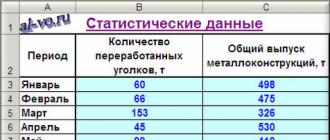
1. We turn on Excel and place a table with statistics data on the sheet.

2. Next, we build and format a scatter plot, in which we set the argument values ​​​​on the X axis - the number of processed corners in tons. On the Y axis, we plot the values ​​of the original function - the total output of metal structures per month, given by the table.

3. “Hover” the mouse over any of the points on the chart and right-click to call up the context menu (as one of my good friends says, when working in an unfamiliar program, when you don’t know what to do, right-click more often ...). In the drop-down menu, select "Add trend line ...".

4. In the "Trend line" window that appears, on the "Type" tab, select "Linear".

6. A straight line appeared on the graph, approximating our tabular dependence.

In addition to the line itself, we see the equation of this line and, most importantly, we see the value of the parameter R 2 - the magnitude of the approximation reliability! The closer its value is to 1, the more accurately the selected function approximates tabular data!

7. We build trend lines using power, logarithmic, exponential and polynomial approximations in the same way as we built a linear trend line.

The polynomial of the second degree best of all of the selected functions approximates our data, it has the maximum reliability coefficient R 2 .

However, I want to warn you! If you take polynomials of higher degrees, you will probably get even better results, but the curves will look intricate…. It is important to understand here that we are looking for a function that has a physical meaning. What does this mean? This means that we need an approximating function that will give adequate results not only within the considered range of X values, but also beyond it, that is, it will answer the question: “What will be the output of metal structures if the number of angles processed per month is less than 45 and more than 168 tons! Therefore, I do not recommend getting carried away with high-degree polynomials, and choose a parabola (polynomial of the second degree) carefully!

So, we need to choose a function that not only interpolates tabular data well within the range of values ​​X = 45 ... 168, but also allows adequate extrapolation outside this range. I choose in this case a logarithmic function, although you can choose a linear one, as the simplest. In the example under consideration, when choosing a linear approximation in excel, the errors will be larger than when choosing a logarithmic one, but not by much.

8. We remove all trend lines from the chart field, except for the logarithmic function. To do this, right-click on unnecessary lines and select "Clear" in the drop-down context menu.

9. Finally, we add error bars to the tabular data points. To do this, right-click on any of the points on the chart and select "Format of data series ..." in the context menu and configure the data on the "Y-errors" tab as shown in the figure below.

10. Then we right-click on any of the lines of error ranges, select "Format of error bars ..." in the context menu and in the "Format of error bars" window on the "View" tab, adjust the color and thickness of the lines.

Any other chart objects are formatted in the same way.excel!

The final result of the chart is presented in the following screenshot.

Results.

The result of all previous actions was the resulting formula for the approximating function y=-172.01*ln (x)+1188.2. Knowing it, and the number of corners in the monthly set of works, it is possible with a high degree of probability (± 4% - see error bars) to predict the total production of metal structures for the month! For example, if there are 140 tons of angles in the monthly plan, then the total output, all other things being equal, will most likely be 338 ± 14 tons.

To increase the reliability of the approximation, there should be a lot of statistical data. Twelve pairs of values ​​is not enough.

From practice I will say that finding an approximating function with a reliability coefficient R 2 >0.87 should be considered a good result. Excellent result - at R 2 >0.94.

In practice, it can be difficult to single out one most important determining factor (in our example, the mass of corners recycled in a month), but if you try, you can always find it in each specific task! Of course, the total output per month really depends on hundreds of factors, which require significant labor costs of rate-setters and other specialists to take into account. Only the result will still be approximate! So is it worth it to bear the cost when there is much cheaper mathematical modeling!

In this article, I have only touched the tip of the iceberg called the collection, processing and practical use of statistical data. Whether I succeeded or not, I stir up your interest in this topic, I hope to learn from the comments and rating of the article in search engines.

The touched upon issue of approximation of the function of one variable has a wide practical application in different spheres of life. But the solution of the problem of approximating the function has a much greater application several independent variables…. Read about this and more in the following blog posts.

Subscribe to announcements of articles in the window located at the end of each article or in the window at the top of the page.

Do not forget confirm subscription by clicking on the link in a letter that will come to you at the specified mail (may come in a folder « Spam » )!!!

I will read your comments with interest, dear readers! Write!

P.S. (06/04/2017)

Highly accurate beautiful replacement of tabular data with a simple equation.

You are not satisfied with the obtained approximation accuracy (R 2<0,95) или вид и набор функций, предлагаемые MS Excel?

Are the dimensions of the expression and the shape of the line of the approximating high-degree polynomial not pleasing to the eye?

Refer through the page " " for a more accurate and compact result of fitting your tabular data and in order to learn a simple technique for solving problems of high-precision approximation by a function of one variable.

When using the proposed algorithm of actions, a very compact function was found that provides the highest approximation accuracy: R 2 =0.9963!!!

Nonlinear Function Approximation

x 0 /12 /6 /4 /3 5/12 /2

y 0.5 0.483 0.433 0.354 0.25 0.129 0

Since the interval of splitting the function is equal, we calculate the following slope coefficients of the corresponding sections of the function being approximated:

1. Building blocks for forming segments of the approximating function

Formation of the time function

Change interval:

Cyclic restart time: T = 1s

Now let's model the function:

Approximation

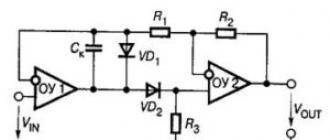
Figure 3.1 - Scheme for solving the equation

Figure 3.2 - Block diagram of the formation of a non-linear function

Thus, the left side of the equation is automatically formed. In this case, it is conventionally considered that the highest derivative x// is known, since the members of the right side of the equation are known and can be connected to the inputs Y1 (Figure 3.1). Operational amplifier U3 acts as an +x signal inverter. To simulate x//, it is necessary to introduce one more subsuming amplifier into the circuit, to the inputs of which it is necessary to apply signals that simulate the right side of equation (3.2).

The scales of all variables are calculated, taking into account that the maximum value of the machine variable behind the absolute value is 10 V:

Mx = 10 / xmax; Mx/ = 10 / x/max; Mx// = 10 / x //max;

My = 10 / ymax. (3.3)

The time scale is Mt = T / tmax = 1, since the simulation of the problem is carried out in real time.

The transmission coefficients are calculated for each input of the integrating amplifiers.

For the U1 amplifier, the transfer coefficients are behind the formulas:

K11 = Mx/b/(MyMt); K12 = Mx/ a2 / (MxMt);

K13 = Mx/ a1 / (MxMt). (3.4)

For amplifier U2:

K21 = Mx/ / (Mx/ Mt), (3.5)

and for amplifier U3:

K31 = 1. (3.6)

The stresses of the initial conditions are calculated using the formulas:

ux/ (0) = Mx/ x/ (0) (-1); ux(0)= Mxx(0) (+1). (3.7)

The right side of equation (3.2) is represented by a non-linear function, which is given by linear approximation. In this case, it is necessary to check that the approximation error does not exceed the specified value. The block diagram of the formation of a non-linear function is shown in Figure 3.2.

Circuit diagram description

The time function (F) generation unit is made in the form of one (to form t) or two series-connected (to form t2) integrating amplifiers with zero initial conditions.

In this case, when the signal U is applied to the input of the first integrator, at its output we get:

u1(t)= - K11 = - K11Et. (3.8)

Setting K11E=1, we have u1(t)= t.

At the output of the second integrator we get:

u2(t)= K21 = K11K21Et2 / 2 (3.9)

Setting K11K21E/2 = 1, we have u2(t)= t2.

Blocks for forming segments of the approximating function are implemented in the form of diode blocks of nonlinear functions (DBNF), the input value for which is a function of time t or t2. The procedure for calculating and constructing DBNF is given in.

The adder (SAD) of segments of the approximating function is implemented as a differential final amplifier.

The initial conditions for the integrators of the modeling circuit are introduced using a node with a variable structure (Figure 3.3). This scheme can work in two modes:

a) integration - with the position of the key K in position 1. In this case, the initial signal of the circuit is described with sufficient accuracy by the equation of an ideal integrator:

u1(t)= - (1 / RC) . (3.10)

This mode is used when modeling a task. To check the correctness of the choice of parameters R and C of the integrator, check the value of the initial voltage of the integrator as a function of time and the useful integration time within the allowable error?

The value of the initial voltage of the integrator

U(t)= - KYE (1 - e - T / [(Ky+1)RC) (3.11)

during the simulation time T when integrating the input signal E using an op-amp with gain Ky without feedback loop, must not exceed the value of the machine variable (10 V).

Integration time

Ti \u003d 2RC (Ku + 1)? Uadd (3.12)

for the selected circuit parameters should not be less than the simulation time T.

b) setting the initial conditions is implemented when the key K is set to position 2. This mode is used when preparing the modeling circuit for the solution process. In this case, the initial signal of the circuit is described by the equation:

u0(t)= - (R2 /R1) E (3.13)

where u0(t) is the value of the initial conditions.

In order to reduce the time of formation of initial conditions and ensure reliable operation, the circuit parameters must satisfy the condition: R1C1 = R2C.

Build a complete calculation scheme. In this case, the conventions given in subsection 3.1 should be used.

Using the capacity of the input and source data, construct the schematic diagrams of blocks B1 and B2 and connect them to the PC block.

Among the various forecasting methods, it is impossible not to single out the approximation. With its help, you can make approximate calculations and calculate planned indicators by replacing the original objects with simpler ones. In Excel, there is also the possibility of using this method for forecasting and analysis. Let's look at how this method can be applied in the specified program with built-in tools.

The name of this method comes from the Latin word proxima - “nearest”. It is the approximation by simplifying and smoothing known indicators, lining them up in a trend that is its basis. But this method can be used not only for forecasting, but also for the study of existing results. After all, the approximation is, in fact, a simplification of the initial data, and the simplified version is easier to study.

The main tool with which smoothing is carried out in Excel is the construction of a trend line. The bottom line is that on the basis of existing indicators, the graph of the function for future periods is being completed. The main purpose of the trend line, as you might guess, is making forecasts or identifying a general trend.

But it can be built using one of five types of approximation:

• Linear;
• exponential;
• logarithmic;
• polynomial;
• Power.

Let's consider each of the options in more detail separately.

Method 1: Linear Smoothing

First of all, let's consider the simplest version of approximation, namely using a linear function. We will dwell on it in more detail, as we will state the general points characteristic of other methods, namely, plotting and some other nuances, which we will not dwell on when considering subsequent options.

First of all, let's build a graph, on the basis of which we will carry out the smoothing procedure. To build a graph, let's take a table in which the cost of a unit of output produced by the enterprise and the corresponding profit in a given period are indicated on a monthly basis. The graphical function that we will build will display the dependence of the increase in profit on the decrease in the cost of production.

The smoothing used in this case is described by the following formula:

In our particular case, the formula takes the following form:

y=-0.1156x+72.255

The value of the approximation reliability is equal to 0,9418 , which is a fairly acceptable result characterizing smoothing as reliable.

Method 2: Exponential Approximation

Now let's look at the exponential type of approximation in Excel.

The general form of the smoothing function is as follows:

Where e is the base of the natural logarithm.

In our particular case, the formula took the following form:

y=6282.7*e^(-0.012*x)

Method 3: logarithmic smoothing

Now it is the turn to consider the logarithmic approximation method.

In general, the smoothing formula looks like this:

Where ln is the natural logarithm. Hence the name of the method.

In our case, the formula takes the following form:

y=-62.81ln(x)+404.96

Method 4: Polynomial Smoothing

The time has come to consider the method of polynomial smoothing.

The formula that describes this type of smoothing has taken the following form:

y=8E-08x^6-0.0003x^5+0.3725x^4-269.33x^3+109525x^2-2E+07x+2E+09

Method 5: power smoothing

In conclusion, consider the power approximation method in Excel.

This method is effectively used in cases of intensive change of function data. It is important to note that this option is applicable only if the function and argument do not take negative or zero values.

The general formula describing this method is as follows:

In our particular case, it looks like this:

y = 6E+18x^(-6.512)

As you can see, when using the specific data that we used for the example, the method of polynomial approximation with a sixth degree polynomial showed the highest level of reliability ( 0,9844 ), the lowest level of reliability for the linear method ( 0,9418 ). But this does not mean at all that the same trend will be when using other examples. No, the level of efficiency of the above methods can vary significantly, depending on the specific type of function for which the trend line will be built. Therefore, if the selected method is the most efficient for this function, this does not mean at all that it will also be optimal in another situation.

If you cannot immediately determine, based on the above recommendations, which type of approximation is suitable specifically for your case, then it makes sense to try all the methods. After plotting the trend line and viewing its confidence level, you can choose the best option.

Numerical methods for solving problems

Radio Physics and Electronics

(Tutorial)

Voronezh 2009

The textbook was prepared at the Department of Electronics of the Physical

Faculty of the Voronezh State University.

Methods for solving problems related to automated analysis of electronic circuits are considered. The basic concepts of graph theory are outlined. A matrix-topological formulation of Kirchhoff's laws is given. The most well-known matrix-topological methods are described: nodal potential method, loop current method, discrete model method, hybrid method, state variable method.

1. Approximation of nonlinear characteristics. Interpolation. 6

1.1. Newton and Lagrange polynomials 6

1.2. Spline Interpolation 8

1.3. Least Squares 9

2. Systems of algebraic equations 28

2.1. Systems of linear equations. Gauss method. 28

2.2. Sparse systems of equations. LU factorization. 36

2.3. Solving non-linear equations 37

2.4. Solving Systems of Nonlinear Equations 40

2.5. Differential equations. 44

2. Methods for searching for an extremum. Optimization. 28

2.1. Extremum Search Methods. 36

2.2. Passive search 28

2.3. Sequential search 36

2.4. Multidimensional optimization 37

References 47

Approximation of nonlinear characteristics. Interpolation.

1.1. Polynomials of Newton and Lagrange.

When solving many problems, it becomes necessary to replace the function f, about which there is incomplete information or the form of which is too complex, with a simpler and more convenient function F, close in one sense or another to f, giving its approximate representation. For approximation (approximation), functions F belonging to a certain class are used, for example, algebraic polynomials of a given degree. There are many different variants of the function approximation problem, depending on which functions f are being approximated, which functions F are used for approximation, how the closeness of f and F is understood, and so on.

One of the methods for constructing approximate functions is interpolation, when it is required that at certain points (interpolation nodes) the values ​​of the original function f and the approximating function F coincide. In a more general case, the values ​​of derivatives at given points should coincide.

Function interpolation is used to replace a hard-to-calculate function with another easier-to-compute one; for approximate recovery of a function from its values ​​at individual points; for numerical differentiation and integration of functions; for the numerical solution of nonlinear and differential equations, etc.

The simplest interpolation problem is as follows. For some function on a segment, n + 1 values ​​are given at points , which are called interpolation nodes. Wherein . It is required to construct an interpolating function F(x) that takes the same values ​​at the interpolation nodes as f(x):

F(x 0) \u003d f (x 0), F (x 1) \u003d f (x 1), ..., F (x n) \u003d f (x n)

Geometrically, this means finding a curve of a certain type passing through a given system of points (x i , y i), i = 0,1,…,n.

If the values ​​of the argument go beyond the region, then they speak of extrapolation - the continuation of the function beyond the region of its definition.

Most often, the function F(x) is constructed as an algebraic polynomial. There are several representations of algebraic interpolation polynomials.

One of the methods for interpolating functions that takes values ​​at points is the construction of a Lagrange polynomial, which has the following form:

The degree of the interpolation polynomial passing through n+1 interpolation nodes is n.

It follows from the form of the Lagrange polynomial that adding a new nodal point leads to a change in all members of the polynomial. This is the inconvenience of Lagrange's formula. But the Lagrange method contains the minimum number of arithmetic operations.

To construct Lagrange polynomials of increasing degrees, the following iterative scheme (Aitken's scheme) can be applied.

Polynomials passing through two points (x i , y i) , (x j , y j) (i=0,1,…,n-1 ; j=i+1,…,n) can be represented as follows:

Polynomials passing through three points (x i , y i) , (x j , y j) , (x k , y k)

(i=0,…,n-2 ; j=i+1,…,n-1 ; k=j+1,…,n) can be expressed in terms of polynomials L ij and L jk:

Polynomials for four points (x i , y i) , (x j , y j) , (x k , y k) , (x l , y l) are built from polynomials L ijk and L jkl:

The process continues until a polynomial passing through n given points is obtained.

The algorithm for calculating the value of the Lagrange polynomial at the point XX, which implements the Aitken scheme, can be written using the operator:

for (int i=0;i

for (int i=0;i<=N-2;i++)Здесь не нужно слово int, программа

will perceive it as an error - re-declaration of a variable,

variable i has already been declared

for (int j=i+1;j<=N-1;j++)

F[j]=((arg-x[i])*F[j]-(arg-x[j])*F[i])/(x[j]-x[i]);

where the array F is the intermediate values ​​of the Lagrange polynomial. Initially, F[I] should be set equal to y i . After executing the loops, F[N] is the value of the Lagrange polynomial of degree N at the point XX.

Another form of representation of the interpolation polynomial is Newton's formulas. Let be equidistant interpolation nodes; i=0,1,…,n ; - interpolation step.

Newton's 1st interpolation formula, which is used for forward interpolation, is:

It is called (finite) differences of the i-th order. They are defined like this:

Normalized argument.

At , Newton's interpolation formula turns into a Taylor series.

Newton's 2nd interpolation formula is used to interpolate "backwards":

In the last entry, instead of differences (called “forward” differences), “backward” differences are used:

In the case of unequally spaced nodes, the so-called. divided differences

In this case, the interpolation polynomial in the Newton form has the form

In contrast to the Lagrange formula, the addition of a new pair of values. (x n +1 , y n +1) is reduced here to adding one new term. Therefore, the number of interpolation nodes can be easily increased without repeating the entire calculation. This allows you to evaluate the accuracy of the interpolation. However, Newton's formulas require more arithmetic than Lagrange's formulas.

For n=1, we get the linear interpolation formula:

For n=2 we will have the parabolic interpolation formula:

When interpolating functions, high-degree algebraic polynomials are rarely used due to significant computational costs and large errors in calculating values.

In practice, piecewise linear or piecewise parabolic interpolation is most often used.

With piecewise linear interpolation, the function f(x) on the interval (i=0,1,…,n-1) is approximated by a straight line segment

The calculation algorithm that implements piecewise linear interpolation can be written using the operator:

for (int i=0;i

if ((arg>=Fx[i]) && (arg<=Fx))

res=Fy[i]+(Fy-Fy[i])*(arg-Fx[i])/(Fx-Fx[i]);

Using the first loop, we are looking for where the desired point is located.

In piecewise parabolic interpolation, the polynomial is built using the 3 nodal points closest to the given argument value.

The calculation algorithm that implements piecewise parabolic interpolation can be written using the operator:

for (int i=0;i

y0=Fy; For i=0, the element does not exist!

x0=Fx; The same

res=y0+(y1-y0)*(arg-x0)/(x1-x0)+(1/(x2-x0))*(arg-x0)*(arg-x1)*(((y2-y1) /(x2-x1))-((y1-y0)/(x1-x0)));

The use of interpolation is not always advisable. When processing experimental data, it is desirable to smooth the function. Approximation of experimental dependences by the least squares method proceeds from the requirement of minimizing the mean square error

The coefficients of the approximating polynomial are found from the solution of a system of m + 1 linear equations, the so-called. "normal" equations , k=0,1,…,m

In addition to algebraic polynomials, trigonometric polynomials are widely used to approximate functions.

(see "numerical harmonic analysis").

Splines are an effective apparatus for approximating a function. The spline requires the coincidence of its values ​​and derivatives at nodal points with the interpolated function f(x) and its derivatives up to a certain order. However, the construction of splines in some cases requires significant computational costs.

Characteristics of real non-linear elements, which are usually determined with the help of experimental studies, have a complex form and are presented in the form of tables or graphs. At the same time, for the analysis and calculation of circuits, an analytical representation of the characteristics is necessary, i.e. representation in the form of rather simple functions. The process of compiling an analytical expression for characteristics presented graphically or tabularly is called approximation.

Approximation solves the following problems:

1. Determining the area of ​​approximation, which depends on the range of input signals.

2. Determining the approximation accuracy. It is clear that the approximation gives an approximate representation of the characteristic in the form of some analytical expression. Therefore, it is necessary to quantify the degree of approximation of the approximating function to the experimentally determined characteristic. Most commonly used:

indicator of uniform approximation - the approximating function should not differ from the given function by more than a certain number , i.e.

;

mean square approximation indicator - the approximating function should not differ from the given function in the mean square approximation by more than a certain number, i.e.

;

nodal approximation (interpolation) - the approximating function must coincide with the given function at some selected points.

There are various methods of approximation. Most often, for the approximation of the I–V characteristics, approximation by a power polynomial and piecewise linear approximation is used, less often - approximation using exponential, trigonometric or special functions (Bessel, Hermite, etc.).

7.2.1. Approximation by a power polynomial

The nonlinear current-voltage characteristic in the vicinity of the operating point is represented by a finite number of terms in the Taylor series:

The number of terms in the series is determined by the required approximation accuracy. The more terms in the series, the more accurate the approximation. In practice, the required accuracy is achieved using approximation by polynomials of the second and third degrees. Odds - these are numbers that are quite simply determined from the VAC graph, which is illustrated by an example.

Example.

To approximate the one shown in Fig. 7.1,a CVC in the vicinity of the operating point by a power polynomial of the second degree, i.e. polynomial of the form

Let's choose the area of ​​approximation from 0.2 V to 0.6 V. To solve the problem, it is necessary to determine three coefficients . Therefore, we restrict ourselves to three nodal points (in the middle and at the boundaries of the selected range), for which we compose a system of three equations:

Rice. 7.1. Approximation of the IV characteristics of a transistor

Solving the system of equations, we determine , , . Therefore, the analytical expression describing the I–V curve has the form

Note that the approximation by a power polynomial is mainly used to describe individual fragments of characteristics. With significant deviations of the input signal from the operating point, the accuracy of the approximation may deteriorate significantly.

If the CVC is not specified graphically, but by some analytical function and it becomes necessary to represent it as a power polynomial, then the coefficients are calculated using the well-known formula

.

It is easy to see that is the I–V slope at the operating point. The value of the steepness essentially depends on the position of the operating point.

In some cases, it is more convenient to represent the characteristic by the Maclaurin series

7.2.2. Piecewise linear approximation

If the input signal varies in magnitude over a large range, then the I–V characteristic can be approximated by a broken line consisting of several straight line segments. On fig. 7.1b shows the current-voltage characteristic of the transistor, approximated by three line segments.

Mathematical formula of the approximate CVC

This type of approximation is associated with two important parameters of a non-linear element: the voltage of the beginning of the characteristic and its steepness. To increase the approximation accuracy, increase the number of line segments. However, this complicates the CVC mathematical formula.