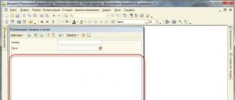
In Excel, there are several options for moving text within one cell.
1 way
You need to use the cell formatting tool.
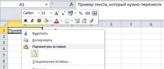
1) Right-click on the desired cell or on several cells at once in which you want to wrap text. From the context menu, select Format Cells.

2) The formatting window opens. You need to open the “Alignment” tab and in the “Display” block check the “Word Wrap” box.

3) All that remains is to click on the “OK” button. The text will be wrapped and will appear not in one line, but in several.

Method 2
1) Select the desired cell; to do this, simply click on it with the left mouse button.
2) On the Excel toolbar, click on the “Text Wrap” button.

This method is much more convenient than the previous one and takes less time.
3 way
1) Go to text editing mode, to do this, double-click the left mouse button inside the cell. The cursor must be placed in front of the part of the text that needs to be moved.

2) Now type the key combination “Alt” + “Enter” on your keyboard. The text will be split.

3) To see the final result, just exit the cell editing mode.

To exit the editing mode, you can press the "Enter" key or click once with the left mouse button on any other table cell.
If you periodically create documents in Microsoft Excel, then you have noticed that all data entered into a cell is written on one line. Since this may not always be suitable, and the option to stretch the cell is also not appropriate, the need arises to wrap the text. The usual “Enter” press is not suitable, since the cursor immediately jumps to a new line, so what should I do next?
In this article, we will learn how to move text in Excel to a new line within one cell. Let's look at how this can be done in various ways.
Method 1
You can use the key combination “Alt+Enter” for this. Place italics in front of the word that should start on a new line, press “Alt”, and without releasing it, click “Enter”. Everything, italics or phrase will jump to a new line. Type all the text in this way, and then press “Enter”.
The bottom cell will be selected, and the one we need will increase in height and the text in it will be fully visible.
To perform some actions faster, check out the list of shortcut keys in Excel.

Method 2
To ensure that while typing words, italics automatically jump to another line when the text no longer fits in width, do the following. Select a cell and right-click on it. In the context menu, click Format Cells.

At the top, select the “Alignment” tab and check the box next to the item "translate according to words". Click "OK".

Write everything you need, and if the next word does not fit in width, it will start on the next line.
If in a document lines must be wrapped in many cells, then first select them, and then check the box mentioned above.

Method 3
In some cases, everything that I described above may not be suitable, since it is necessary that information from several cells be collected in one, and already divided into lines in it. So let's figure out what formulas to use to get the desired result.
One of them is CHAR() . Here, in brackets, you need to indicate a value from one to 255. The number is taken from a special table, which indicates which character it corresponds to. To move a line, code 10 is used.
Now about how to work with the formula. For example, let's take data from cells A1:D2 and write what is written in different columns (A, B, C, D) in separate lines.
I put italics in the new cell and write in the formula bar:
A1&A2&CHAR(10)&B1&B2&CHAR(10)&C1&C2&CHAR(10)&D1&D2
We use the “&” sign to concatenate cells A1:A2 and so on. Press "Enter".

Don't be afraid of the result - everything will be written in one line. To fix this, open the “Format Cells” window and check the transfer box, as described above.

As a result, we will get what we wanted. The information will be taken from the specified cells, and where CHAR(10) was entered in the formula, a transfer will be made.

Method 4
To transfer text in a cell, another formula is used - . Let's take only the first line with the headings: Last Name, Debt, Payable, Amount. Click on an empty cell and enter the formula:
CONCATENATE(A1,CHAR(10),B1,CHAR(10),C1,CHAR(10),D1)
Instead of A1, B1, C1, D1, indicate the ones you need. Moreover, their number can be reduced or increased.

The result we will get is this.

Therefore, open the already familiar Format Cells window and mark the transfer item. Now the necessary words will begin on new lines.

In the next cell I entered the same formula, only I indicated other cells: A2:D2.
The advantage of using this method, like the previous one, is that when the data in the source cells changes, the values in these will also change.
In the example, the debt number has changed. If you also automatically calculate the amount in Excel, then you won’t have to change anything else manually.

Method 5
If you already have a document in which a lot is written in one cell, and you need to move words, then we will use the formula.

The gist of it is that we will replace all spaces with a line break character. Select a blank cell and add the formula to it:
SUBSTITUTE(A11;" ";CHAR(10))
Instead of A11 there will be your original text. Press the “Enter” button and immediately each word will be displayed on a new line.

By the way, in order not to constantly open the Format Cells window, you can use a special button "Move text", which is located on the "Home" tab.

I think the methods described are enough to move italics to a new line in an Excel cell. Choose the one that is most suitable for solving the task.
As you know, by default, one cell of an Excel sheet contains one row with numbers, text or other data. But what if you need to move text within one cell to another line? This task can be accomplished using some of the program's features. Let's figure out how to make a line feed in a cell in Excel.
Some users try to move text inside a cell by pressing a button on the keyboard Enter. But by doing this they only achieve that the cursor moves to the next line of the sheet. We will consider transfer options within the cell, both very simple and more complex.
Method 1: Using the Keyboard
The easiest way to move to another line is to place the cursor in front of the segment that needs to be moved, and then type the key combination on the keyboard Alt+Enter.

Unlike using only one button Enter, using this method, exactly the desired result will be achieved.

Method 2: Formatting
If the user is not tasked with moving strictly defined words to a new line, but only needs to fit them within one cell without going beyond its boundaries, then you can use the formatting tool.


After this, if the data extends beyond the boundaries of the cell, it will automatically expand in height and the words will begin to wrap. Sometimes you have to expand the boundaries manually.
To avoid formatting each individual element in this way, you can select an entire area at once. The disadvantage of this option is that the transfer is performed only if the words do not fit within the boundaries, and the division is carried out automatically without taking into account the user’s wishes.
Method 3: Using a Formula
You can also carry out transfer within a cell using formulas. This option is especially relevant if the content is output using functions, but it can be used in ordinary cases.


The main disadvantage of this method is the fact that it is more difficult to implement than previous options.
In general, the user must decide for himself which of the proposed methods is best to use in a particular case. If you only want all the characters to fit within the boundaries of the cell, then simply format it as necessary, or it is best to format the entire range. If you want to transfer specific words, then type the appropriate key combination, as described in the description of the first method. The third option is recommended to be used only when data is pulled from other ranges using a formula. In other cases, the use of this method is irrational, since there are much simpler options for solving the problem.
Quite often the question arises, how to move to another line inside a cell in Excel? This question arises when the text in a cell is too long, or when wrapping is necessary to structure the data. In this case, it may not be convenient to work with tables. Typically, text is transferred using the Enter key. For example, in Microsoft Office Word. But in Microsoft Office Excel, when we press Enter, we go to the adjacent lower cell.
So we need to wrap the text to another line. To transfer, you need to press the keyboard shortcut Alt+Enter. After which the word located on the right side of the cursor will be moved to the next line.
Automatically wrap text in Excel
In Excel, on the Home tab, in the Alignment group, there is a “Text Wrap” button. If you select a cell and click this button, the text in the cell will wrap to a new line automatically depending on the width of the cell. Automatic transfer requires a simple click of a button.

Remove hyphen using function and hyphen symbol
In order to remove the carry, we can use the SUBSTITUTE function.
The function replaces one text with another in the specified cell. In our case, we will replace the space character with a hyphen character.
Formula syntax:
SUBSTITUTE (text; old_text; new_text; [occurrence number])
The final form of the formula:
SUBSTITUTE(A1,CHAR(10), " ")
- A1 – cell containing hyphenated text,
- CHAR(10) – line break character,
- » » – space.

If, on the contrary, we need to insert a hyphen to another line, instead of a space, we will perform this operation in reverse.
SUBSTITUTE(A1; ";CHAR(10))
For the function to work correctly, the “Wrap by words” checkbox must be checked in the Alignment tab (Cell Format).
Transfer using the CONCATENATE formula
To solve our problem, we can use the CONCATENATE formula.
Formula syntax:
CONCATENATE (text1,[text2]…)
We have text in cells A1 and B1. Let's enter the following formula in B3:
CONCATENATE(A1,CHAR(10),B1)

As in the example I gave above, for the function to work correctly, you need to set the “word wrap” checkbox in the properties.
In this lesson we will learn useful Microsoft Excel functions such as wrapping text across lines and merging multiple cells into one. Using these functions, you can wrap text on multiple lines, create headings for tables, enter long text on one line without increasing the width of the columns, and much more.
Very often the content cannot be completely displayed in the cell, because... its width is not enough. In such cases, you can choose one of two options: move text across rows or combine several cells into one, without changing the width of the columns.
When text wraps, the line height will automatically change, allowing content to appear on multiple lines. Merging cells allows you to create one large cell by merging several adjacent ones.
In the following example, we will apply line wrapping to column D.
Click command Wrap text again to cancel the transfer.
When two or more cells are merged, the resulting cell takes the place of the merged cell, but the data is not added. You can merge any adjacent range, and even all cells on a worksheet, and the information in all cells except the top left will be deleted.
In the example below, we'll concatenate the range A1:E1 to create a title for our sheet.

The button acts as a switch, i.e. Clicking it again will cancel the merge. Deleted data will not be restored
More options for merging cells in Excel
To access additional options for merging cells, click the arrow next to the command icon Combine and place in the center. A drop-down menu will appear with the following commands: