If you read to the end, you will learn how to use such a useful Excel function as filter... Now, with a very real example, I will show what Excel filters are and how to save time when working with large tables. It's not difficult at all. At the end of the article, you can download a spreadsheet, which I use here as an example of working with Excel filters.
Why do you need filters in Excel tables
And then to be able to quickly select only the data you need, hiding unnecessary strings tables. Thus, the filter allows without deleting Excel table rows just temporarily hide them.
The rows of the table hidden by the filter do not disappear. You can conditionally imagine that their height becomes equal to zero (I talked about changing the height of the rows and the width of the columns). Thus, the rest of the lines not hidden by the filter seem to be "glued together". The result is a filtered table.
Databases are very convenient for storing information, but we create them in order to receive the information we need when the need arises.
For example, we need a schedule of train trains that leave for Moscow on Friday after 4 pm, etc.
The search for the required information is carried out by selecting rows that meet a certain criterion. In most cases, the selection criterion is the equality of the cell content to a certain value.
In addition to comparing for equality, you can use other comparison operations when selecting records. For example, greater, less, greater or equal, less than or equal. Using these operations allows you to formulate the query criterion less rigorously. For example, if you need to find information about a person whose last name begins with "Ku", then as a criterion, you can use the rule "the content of the Last name cell is greater than or equal to Ku and the content of the Last name cell is less than L".
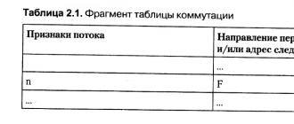
The process of selecting rows from a table that satisfy a certain criterion (rule) is called filtering, and the criterion (condition for selecting rows) is called a filter.
- In order to select rows from the table that satisfy a certain condition, you need:
- 1. Select the table row that contains the column names, open the Home -\u003e Editing tab and select the Filter command in the Sort and Filter list. As a result, drop-down list buttons will appear in the selected row, next to the table column names.
- 2. Expand the list by clicking on the column heading, and in the opened window, first clear the switch (Select all), then select the value that should be used as a criterion for selecting rows.


As a result of performing the above actions, only those rows that satisfy the query condition will remain on the screen.

As a criterion for selecting a column that contains numeric values, you can specify the range in which the cell values \u200b\u200bshould be. For example, to get a list of expenses, the amount of which lies in the range of 100 rubles. up to 1000 rubles, you need to open the filter window for the Amount column, select Numeric filters -\u003e between and enter the range boundaries in the Custom AutoFilter window that appears.


You can display information on one / several parameters by filtering data in Excel.
There are two tools for this purpose: AutoFilter and Advanced Filter. They do not delete, but hide data that does not match the condition. An autofilter performs the simplest operations. The advanced filter has many more options.
Auto filter and advanced filter in Excel
There is a simple table, neither formatted nor declared as a list. You can enable the automatic filter through the main menu.

If you format the data range as a table or declare it as a list, then the automatic filter will be added immediately.
Using the AutoFilter is simple: you just need to select the entry with the desired value. For example, display deliveries to store # 4. We put a checkbox opposite the corresponding filtration condition:

We immediately see the result:
Features of the tool:
- The autofilter works only in the continuous range. Different tables on one sheet are not filtered. Even if they have the same type of data.
- The tool treats the top line as column headings - these values \u200b\u200bare not included in the filter.
- Several filtering conditions can be applied at once. However, each previous result can hide the records needed for the next filter.
The advanced filter has many more options:
- You can set as many filtering conditions as needed.
- Data selection criteria are visible.
- Using the advanced filter, the user can easily find unique values \u200b\u200bin a multi-line array.
How to make an advanced filter in Excel
A finished example - how to use the advanced filter in Excel:


Only the rows containing the value "Moscow" remain in the original table. To cancel filtering, you need to click the "Clear" button in the "Sort and Filter" section.
How to use the advanced filter in Excel
Let's consider using the advanced filter in Excel to select rows containing the words "Moscow" or "Ryazan". Filtering conditions must be in one column. In our example, under each other.

Fill in the advanced filter menu:

We get a table with rows selected according to a given criterion:

Let's select the rows that contain the value “# 1” in the “Store” column, and “\u003e 1,000,000 rubles” in the cost column. The filtering criteria must be in the appropriate columns of the condition plate. On one line.

Fill in the filtering parameters. Click OK.
Let's leave in the table only those rows that contain the word “Ryazan” in the “Region” column or the value “\u003e 10,000,000 rubles” in the “Cost” column. Since the selection criteria refer to different columns, we place them on different lines under the appropriate headings.

Let's apply the Advanced Filter tool:

This tool can work with formulas, which allows the user to solve almost any problem when selecting values \u200b\u200bfrom arrays.
Basic Rules:
- The result of the formula is the selection criterion.
- The written formula returns TRUE or FALSE.
- The original range is indicated using absolute references, and the selection criterion (in the form of a formula) is indicated using relative references.
- If the return value is TRUE, the string will be displayed after the filter is applied. FALSE - no.
Let's display the lines containing the quantity above the average. To do this, aside from the table with the criteria (in cell I1), enter the name "Most". Below is the formula. We use the AVERAGE function.

Select any cell in the original range and call the "Advanced Filter". We indicate I1: I2 as a selection criterion (references are relative!).
Only those rows remained in the table where the values \u200b\u200bin the "Quantity" column were above the average.

To leave only non-repeating rows in the table, in the "Advanced filter" window, check the box next to "Unique records only".

Click OK. Duplicate lines will be hidden. Only unique records will remain on the sheet.
Sometimes Excel spreadsheets contain a fairly large amount of data, for example, a list of consumables purchased per year. And you need to find among them only data related to your department. How to do it?
In order to select only the part that meets your condition from the total mass of records, you can use a tool called a filter. To set a filter, select the headers in the table header or the entire table with the mouse, then on the tab home click on the button Sort and filter and in the menu that appears, select Filter... Downward arrow buttons appear in the lower right corner of the cells with the table column headers, as shown in Fig. 5.4.
If you click on such a button, a menu will appear in which you can specify the direction of sorting by this column, as well as the conditions for selecting records (Fig. 5.5).

If, for example, you need to select only names starting with the letter C in the list, click on the button in the column with names, in the menu that appears, open the Text Filters submenu and select begin with... The window shown in Fig. 5.6. In the field to the right of words starts with, enter the letter C. You can enter more than one letter. As a result, only those names will be selected that begin with the specified combination of letters, and the rest of the table entries will be hidden from the screen (Fig. 5.7).

The button in the cell with the heading of the column on which the filter is set changes and takes the appropriate form. If you click on the button in the column with numeric data, instead of the item Text Filters the menu item appears Number Filters... When you select such an item, you can specify the range of values \u200b\u200bof numbers for the selected records (Fig. 5.8). You can select all records greater than or less than the value you specify.

For the example we are considering (see Figure 5.4), let's select a list of people born after 1973. To do this, click on the button in cell E1 (Year of birth), in the menu that appears, open the submenu Number Filtersas shown in fig. 5.8, and select the item larger. The window shown in Fig. 5.9. In the field to the right of the word more, enter the value 1973 and click the OK button. As a result, only people born after 1973 will remain on the list (Figure 5.10).


The filter can be changed or removed at any time. To do this, click on the button and in the menu that appears, select the item Remove filter from column.

Filtering Excel data includes two filters: AutoFilter and Advanced Filter. Suppose you have a large data set, but from the entire array you need to view or select data that relates to a specific date, a specific person, etc. There are filters for this. For those who come across this tool for the first time, the filter does not delete, but hides records that do not meet the filtering conditions that you specify for them.
The first one is an autofilter, intended for the most simple operations - highlighting records with a specific value (for example, only highlighting only records related to LeBron James), data lying in a certain range (or above the average or top ten) or cells / fonts of a certain color ( by the way, very convenient). Accordingly, it is very easy to use. You just need to select the data that you want to see filtered. Then the command "Data" / "Filter". A list checkbox will appear on each top cell of the top table, it is already easy to understand each command, it is simple to learn and explain, I hope, there is no need for further, only the nuances of using the autofilter:
1) Only works with a continuous range. It will no longer be possible to filter two different lists on one sheet.
2) The topmost row of the table is automatically assigned as a header and does not participate in filtering.
3) You can apply any filters in different columns, but keep in mind that depending on the order in which the filters are applied, some conditions may not be applied. the previous filters have already hidden the required entries. There is no problem here, these entries would be hidden anyway, but if you want to use multiple sets of filters, it is better to start with the conditions that have the least application.
Practical application in work: for example, you work on this list to find an error or check data. After applying the autofilter, you can go through the entire table one by one, sequentially marking the data that has already been viewed. The buttons "Clear" and "Reapply" determine the appearance of the table after applying the conditions. Then, after finishing work with the table, you can return the fonts back to their original appearance without changing the data itself. By the way, some are confused by the fact that all records in the table disappear after applying any conditions. Well, take a closer look, you have specified conditions under which there are no records that meet these conditions. The fact that the table is filtered is that the table row numbers are highlighted in blue.
Now, let's move on to the advanced filter. It differs from the autofilter in more fine tuning, but also in a larger choice when filtering data. In particular:
1) Sets as many conditions as needed.
2) Allows to select cells with unique (non-repeating) data. This is often needed when working with data and the option does an excellent job with the problem.
3) Allows you to copy the filter result to a separate place without touching the main array.

So, the main difference in working with this filter is that we first need to prepare a table of conditions. It is done simply. The headings of the main table are copied and inserted into a convenient place for us (I suggest above the main table). There should be so many lines in this table so that, after defining the conditions, you do not get into the main table.
Examples of conditions:
1) ‘L *’ - cells starting with L
2) ‘\u003e 5’ - data greater than 5
If you delete rows from a filtered table, they will be deleted without taking neighbors with you. Those. if the table is filtered and shows lines 26-29 and 31-25, selecting all lines and deleting them will not delete line 30. This is convenient, personally I often use it when writing macros. What is the advantage of this - often we get tables that need to be brought into working form, i.e. delete, for example empty lines. What we do: filter the table, showing only the rows we don't need, then delete the entire table, including the title. Unnecessary rows and title are removed, and the table has no spaces and is a single range. A header row can be added with simple copy operations from a pre-prepared area. Why is this important when writing macros? It is not known which row the unwanted data starts from and it is not clear which row to start deleting from, deleting the entire table helps to quickly solve this problem.