II. Network model

III. Relational model
recordingfield
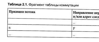
hierarchical and network models foreign keys
4. Relational data model
Relational database
* Attitude
* Attribute columns (fields) tables.
* Data type
* Communication key.
* An association
The main functions The RDBMS are:
· Data definition
· Data processing
· Data management
Microsoft Access
Database window in Access
 |
Modes of working with objects
Buttons for working with database objects are located on the Toolbar of the database window:
Open - allows you to switch to the mode of editing a table, executing a query, loading a form, building a report, running a macro.
Constructor - provides a transition to the setting mode of the selected object.
Create a - allows you to start creating a new object of the selected type.
7. Working with tables
To create a table, you need to go to the list of tables and click the button Create a ... A new dialog will appear New table:

You can create a table in Access in several ways:
· Build a new table "from scratch" using Constructor;
· Run Table Wizard - a special program offering to create a table in a step-by-step mode based on standard solutions available in Access;
· Import a database table from a file of any program, for example, FoxPro or Excel.
Setting the field name
The field name is set in the column Field name... The name can be up to 64 characters long, and any characters other than the period, exclamation point, and angle brackets are allowed. Duplicate field names are not allowed.
Data type definition
For each field, you must specify the type of data it contains. The data type is selected from a list that can be called up by clicking in the column Data type... Access operates on the following data types:
Ø Text- for storing plain text with a maximum of 255 characters.
Ø MEMO field - for storing large amounts of text up to 65,535 characters.
Ø Numerical- for storing real numbers.
Ø Date Time - to store calendar dates and current time.
Ø Monetary- these fields contain monetary amounts.
Ø Counter - to define a unique system key for a table. Typically used for sequential numbering of records. When a new record is added to the table, the value of this field is increased by 1 (one). The values \u200b\u200bin such fields are not updated.
Ø Boolean - for storing data, taking values: Yes or No.
Ø OLE Object Field - for storing objects created in other applications.
Description of field properties
As already noted, the characteristics of individual fields are defined in the field of field properties (tab Are common). Each field has a specific set of properties, depending on the type of field. Some field types have similar sets of field properties. The main properties of the fields are listed below.
Ø Field size - the maximum length of the text field (50 characters by default) or the data type of the numeric field. We recommend that you set this property to the minimum value allowed because smaller data is processed faster.
If the data type is numeric, the following property values \u200b\u200bare valid Field size:
Comment... Data loss may occur if the field is converted to a smaller size.
Ø Field format - the format for displaying data on the screen or printing. Typically, the default format is used.
Ø Decimal places - sets the number of decimal places after the decimal point for the numeric and currency data types.
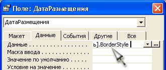
Ø Input mask - defines the form in which data is entered into the field (data entry automation tool).
Ø Signature - designation for a field that will be used to display the field in a table, form or report. If this value is not specified, the field name will be taken as the signature.
Ø Default value - a standard value that is automatically entered into the field when a new data record is generated.
Ø Condition on value- sets restrictions on the entered values, thereby allowing control over the correctness of data entry.
Ø Error message - sets the text of the message displayed on the screen in case of violation of the condition on the value.
Ø Required field- determines whether this field can contain Null values \u200b\u200b(i.e. remain empty), or whether data must be entered into this field.
Ø Indexed field - is used for operations of searching and sorting records by the value stored in this field, as well as for automatic elimination of duplicate records. Type fields MEMO, OLE Object and Hyperlink cannot be indexed.
Defining a key field
After specifying the characteristics of all fields, you must select at least one key field. As a rule, fields that have non-repeating data are specified as key fields or fields with a data type are created Counter ... In any case, the key field must not contain duplicate data. To define a key, select the required field (or fields) and press the button Key field Edit ... A key image will appear to the left of the marker.
Saving a table
Before entering information, the projected table must be saved: press the button Save on the toolbar or the corresponding command in p.m. File and enter the name of the table, after which the question "Create a key field now?" (Yes or no)
If the answer is “ Yes", Then Access will automatically create a field named" Code "and data type Counter , if a " No", - the table will be created without the key field. In this case, you need to open the created table in the mode Constructor and define "manually" the key field.
Data input
To switch the table to the information input mode, you need to switch to the Tables... The fields are filled in sequentially. It is convenient to move from one field to another by pressing Tab (or a combination Shift + Tab - in the opposite direction). If the table was designed with default values \u200b\u200bfor some of the fields, these values \u200b\u200bwill automatically appear in the corresponding fields. Records in a table can be moved, copied, and deleted in the same ways as in spreadsheets, that is, first select the rows, and then perform the required operation. A column can be selected by clicking on the header. Columns can be moved right and left using the method drag and drop (drag and drop).
If necessary, you can return to the mode Constructor... This makes it possible to correct something in the structure of the table.
Sorting data in a table
The data in the table can be sorted in ascending or descending order. To do this, you need to place the mouse cursor in any cell of the column, the values \u200b\u200bof which will be sorted from the item. Recordings select team Sorting or press the corresponding button on the panel.
8. Creating links between database tables
The relationship between tables is established by defining in one table ( subordinate) of the field corresponding to the key of another table ( the main). The established link will link the records containing the same values \u200b\u200bin the given field. The links that you create are later used by Access in queries, forms, or reports.
Remarks.
Ø Both linked fields must have the same data type.
Ø Properties Field size for both linked fields numeric type should be the same.
Ø If the key field of the main table is a field with a data type Counter, then this field can be associated with a numeric field in a subordinate table. Moreover, for a numeric field of a related table for the property Field size must be set to Long integer .
Data integrity
Data integrity Is a set of rules that maintain correct relationships between records in related tables and protect data from accidental changes or deletions.
These rules include:
Ø In the subordinate table, you cannot enter records that are not related to the record of the main table.
Ø In the main table, you cannot change the value of a key field if there are records in the subordinate table that are associated with it.
Ø Records cannot be deleted in the master table if there are records associated with it in the subordinate table.
Cascading operations
Data integrity in linked tables is ensured by two types of cascading operations:
Ø cascading update operations;
Ø cascading delete operations.
These operations can be turned on and off by selecting the corresponding check boxes: "Cascade update of linked fields" and "Cascade deletion of linked fields".
If the checkbox "Cascading update of related fields" is selected, then any changes in the value of the key field in the main table, which is on the "one" side in the 1: M relationship, will automatically update the corresponding values \u200b\u200bin all related records.
When you select the Cascade Delete Linked Tables check box when deleting a record from the master table, the linked records in the subordinate tables are automatically deleted.
Removing (changing) links
Ø Open window Data schema;
Ø activate the link to be deleted (changed) with the left mouse button;
Ø Right-click to bring up the context-sensitive menu and select the command Delete (Edit) respectively.
9. Types of relationships between tables
There are three types of relationships between tables:
One-to-one (1: 1). The key value in each record in the master table can correspond to the values \u200b\u200bin the associated field in only one record in the subordinate table. In this case, the relationship between the tables can only be established through the key fields of both tables.
One-to-many (1: M). The key value in each record in the master table can correspond to values \u200b\u200bin the associated field (s) in multiple records in the subordinate table. This type of relationship is used quite often in relational databases.
Many-to-many (M: M). Occurs between two tables when one record from the first table A (output link) can be associated with more than one record of another table B (receiving), in turn, one record from another table can be associated with more than one record of the first table ... This scheme is implemented only with the help of the third junction table, the link key of which consists of at least two fields. These fields are foreign key fields in tables A and B. The primary key for a join table is usually a combination of foreign keys.
If there are links of the M: M type between the tables, an additional intersection table is created, with the help of which the M: M relationship will be reduced to two links of the 1: M type. Access does not allow you to define a direct M: M relationship between two tables.
10. Formation of requests
Running a request
To launch an execution request from a window Constructor you need to click on the toolbar button " Running» ! or execute the command Request / Run... The results of data sampling on demand are displayed in the table mode.
Formation of selection conditions
The list of operators used when specifying expressions is as follows:
Ø operators comparisons:
= (equally)
<> (not equal)
> (more)
>= (not less)
< (less)
<= (not more)
BETWEEN - allows you to set a range of values. Syntax: Between"Expression" And"Expression" (for example: BETWEEN 10 And 20 means the same as boolean expression >= 10 AND<= 20).
IN - allows you to specify a list of values \u200b\u200bused for comparison (the operand is a list enclosed in parentheses). For instance: IN("Brest", "Minsk", "Grodno") means the same as the logical expression "Brest" OR "Minsk" OR "Grodno".
Ø brain teaser operators:
AND (for example:\u003e \u003d 10 AND<=20)
OR(eg:<50 OR >100)
NOT(for example: Is Not Null is a field containing some value).
Ø operator LIKE- checks compliance text or Memo fields by a given character pattern.
Template Symbol Table
Examples of using the operator Like:
LIKE "C *" - lines starting with the C character;
LIKE "[A - Z] #" - any character from A to Z and a digit;
LIKE "[! 0 - 9 ABC] * # #" - lines starting with any character except a digit or letters A, B, C and ending with 2 digits;
Complex sampling criteria
Often you have to select records by a condition, which is set for several fields of a table or by several conditions for one field. In this case, apply "I-queries" (select records only if all conditions are met) and OR queries (selection of records when at least one of the conditions is met).
When setting “ OR query»Each selection condition should be placed on a separate line Request form.
When setting “ I-query»Each selection condition must be placed on one line, but in different fields Request form.
These operations can be specified explicitly using the operators OR and AND respectively.
Iif () and Format () Functions
Function IIf (condition; ifTrue; ifFalse) - returns one of two arguments depending on the result of evaluating the expression.
Function Format (expression; format statement) - returns a string containing an expression formatted according to the formatting instructions.
For expressions date / time you can use the following characters in a formatting statement:
I. Hierarchical model
II. Network model
III. Relational model
In the relational model, information is presented in the form of rectangular tables. Each table consists of rows and columns and has a name that is unique within the database. In turn, each line ( recording) of such a table contains information related to only one specific object, and each column ( field) a table has a name unique to its table.
Relational databases (RDBs), as opposed to hierarchical and network models, allow you to organize relationships between tables at any time. For this, the RDB has implemented a mechanism foreign keys... Each database table contains at least one field that serves as a link to another table. In RDB terminology, such fields are called foreign key fields. Using foreign keys, you can link any database tables at any stage of working with the database.
4. Relational data model
Relational database (RDB) is a collection of the simplest two-dimensional logically interconnected relationship tables, consisting of a set of fields and records that reflect a certain subject area.
The relational data model was proposed by E. Codd, a well-known American database specialist. The basic concepts of this model were first published in 1970. As a mathematician by training, Codd proposed using the apparatus of set theory (union, intersection, difference, Cartesian product) for data processing. He showed that any representation of data is reduced to a set of two-dimensional tables of a special kind, known in mathematics as a relation (in English - relation, hence the name - relational databases).
One of Codd's main ideas was that the relationship between data should be established in accordance with their internal logical relationship. The second important principle proposed by Codd is that in relational systems, one command can process entire data files, while previously only one record was processed by one command.
Basic concepts of relational databases (RDBs)
* Attitude - information about objects of the same type, for example, about customers, orders, employees. In a relational database, a relationship is stored as a table.
* Attribute - a certain piece of information about a certain object - for example, a client's address or an employee's salary. The attribute is usually stored as columns (fields) tables.
* Data type - a concept that in the relational model is fully equivalent to the corresponding concept in algorithmic languages. The set of supported data types is determined by the DBMS and can vary greatly from system to system.
* Communication - the way in which information in one table is related to information in another table. Links are made using matching fields called key.
* An association - the process of joining tables or queries based on the matching values \u200b\u200bof certain attributes.
Rules (normalization) for building a relational database
Normalization is a process of data reorganization by eliminating repetitive groups and other contradictions in order to bring tables to a form that allows for consistent and correct editing of data. The ultimate goal of normalization is to get a database design in which each fact appears in only one place, i.e. redundancy of information is excluded.
1. Each field of any table must be unique.
2. Each table must have a unique identifier ( primary key), which can consist of one or more table fields.
3. For each value of the primary key, there must be one and only one value of any of the data columns, and this value must relate to the table object (i.e., the table must not contain data that does not belong to the object defined by the primary key, but also the information in the table should fully describe the object).
4. It should be possible to change the values \u200b\u200bof any field (not included in the primary key), and this should not entail changing another field (ie, there should be no calculated fields).
5. Database management systems (DBMS)
The maintenance of databases in a computer environment is carried out by software tools - database management systems, which are a set of software and language tools for general or specialized purposes necessary for creating databases on machine media, keeping them up to date and organizing access different users to them in the conditions of the adopted data processing technology.
DBMS - these are control programs that provide all manipulations with databases: creating a database, maintaining it, using it by many users, etc., i.e., they implement a complex set of functions for centralized database management and serve the interests of users.
The DBMS can be thought of as a software shell that sits between the database and the user. It provides centralized control of data protection and integrity, access to data, their processing, reporting on the basis of a database, and other operations and procedures.
Relational Database Management System (RDBMS)
A set of tools for managing RDBs is called relational database management system which can contain utilities, applications, services, libraries, application creation tools, and other components. Being linked by means of common key fields, information in the RDB can be combined from many tables into a single result set.
The main functions The RDBMS are:
· Data definition - what information will be stored, set the structure of the database and their type.
· Data processing - you can select any fields, sort and filter data. You can combine data and summarize.
· Data management - correct and add data.
6. General characteristics of DBMS ACCESS
Microsoft Access Is a functionally complete relational DBMS, which provides all the necessary tools for defining and processing data, as well as for managing them when working with large amounts of information. Its various versions are included in the MS Office software package and work in the Windows environment (3.11 / 95/98/2000 / XP).
Database window in Access
After creating a new database file or opening an existing Access window in the workspace, the database window appears:
| |
The advent of computer technology in our time has marked an information revolution in all spheres of human activity. But in order to prevent all information from becoming unnecessary garbage on the global Internet, a database system was invented, in which materials are sorted, systematized, as a result of which they are easy to find and present to subsequent processing. There are three main types - relational databases, hierarchical, network.
Fundamental models
Returning to the emergence of databases, it is worth saying that this process was quite complex, it originates with the development of programmable information processing equipment. Therefore, it is not surprising that the number of their models currently reaches more than 50, but the main ones are hierarchical, relational and network models, which are still widely used in practice. What are they?
Hierarchical has a tree structure and is composed of data from different levels, between which there are links. The DB network model is a more complex pattern. Its structure resembles a hierarchical one, and the scheme is expanded and improved. The difference between them is that the hereditary data of a hierarchical model can have a connection with only one ancestor, while the network data can have several. The structure of a relational database is much more complex. Therefore, it should be analyzed in more detail.
Basic concept of a relational database
Such a model was developed in the 1970s by Edgar Codd, Ph.D. It is a logically structured table with fields describing data, their relationships with each other, operations performed on them, and most importantly - the rules that guarantee their integrity. Why is the model called relational? It is based on relationships (from lat. Relatio) between data. There are many definitions for this type of database. Relational tables with information are much easier to organize and process than in a network or hierarchical model. How can this be done? It is enough to know the features, the structure of the model and the properties of relational tables.

The process of modeling and drawing up the main elements
In order to create your own DBMS, you should use one of the modeling tools, think over what information you need to work with, design tables and relational single and multiple relationships between data, fill in entity cells and set primary, foreign keys.
Table modeling and relational database design is done through free tools such as Workbench, PhpMyAdmin, Case Studio, dbForge Studio. After detailed design, you should save the graphically finished relational model and translate it into ready-made SQL code. At this stage, you can start working with data sorting, processing and systematization.

Features, structure, and terms related to the relational model
Each source describes its elements in its own way, so for less confusion I would like to give a small hint:
- relational label \u003d entity;
- layout \u003d attributes \u003d field names \u003d entity column headers;
- entity instance \u003d tuple \u003d record \u003d table row;
- attribute value \u003d entity cell \u003d field.

To get to the properties of a relational database, you need to know what basic components it consists of and what they are for.
- Essence. A relational database table can be one, or there can be a whole set of tables that characterize the described objects due to the data stored in them. They have a fixed number of fields and a variable number of records. A relational database model table is composed of strings, attributes, and a layout.
- Record - a variable number of lines displaying data that characterize the described object. The records are numbered automatically by the system.
- Attributes are data that demonstrates the description of entity columns.
- Field. Represents an entity column. Their number is a fixed value set during table creation or modification.

Now, knowing the constituent elements of the table, you can go to the properties of the database relational model:
- Relational database entities are two-dimensional. Thanks to this property, it is easy to perform various logical and mathematical operations with them.
- The order of values \u200b\u200bof attributes and records in a relational table can be arbitrary.
- A column within one relational table must have its own individual name.
- All data in an entity column has a fixed length and the same type.
- Any record is in essence considered one data item.
- The constituent components of strings are one of a kind. There are no duplicate rows in a relational entity.
Based on the properties, it is clear that the attribute values \u200b\u200bmust be of the same type and length. Let's consider the features of the attribute values.
Basic characteristics of relational database fields
Field names must be unique within the same entity. Relational database attribute or field types describe which category data is stored in entity fields. A relational database field must have a fixed size in characters. The parameters and format of attribute values \u200b\u200bdetermine how the data is corrected in them. There is also such a thing as "mask" or "input pattern". It is intended to define the configuration of data entry into the attribute value. By all means, when you write something wrong in the field, an error message should be issued. Also, some restrictions are imposed on the elements of the fields - conditions for verifying the accuracy and error-free data entry. There is some required attribute value that must be unambiguously populated with data. Some attribute strings can be filled with NULL values. Entering empty data into field attributes is allowed. Like error notification, there are values \u200b\u200bthat are filled in automatically by the system - this is the default data. An indexed field is designed to speed up the search for any data.

2D relational database table schema
For a detailed understanding of the model using SQL, it is best to consider the schema by example. We already know what a relational database is. A record in each table is one data item. To prevent data redundancy, it is necessary to perform normalization operations.
Basic rules for normalizing a relational entity
1. The value of the field name for a relational table must be unique, one of a kind (the first normal form is 1NF).
2. For a table that has already been reduced to 1NF, the name of any non-identifying column must be dependent on the unique identifier of the table (2NF).
3. For the entire table that is already in 2NF, each non-identifying field cannot depend on an element of another unrecognized value (entity 3NF).
Databases: relational relationships between tables
There are 2 main relational tables:
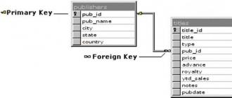
- One-Many. Occurs when one key record of table # 1 matches several instances of the second entity. A key icon at one end of the drawn line indicates that the entity is on the "one" side, the other end of the line is often marked with an infinity symbol.

- A "many-many" relationship is formed when there is an explicit logical interaction between several rows of one entity with a number of records in another table.
- If there is a one-to-one concatenation between two entities, this means that the key identifier of one table is present in another entity, then one of the tables should be removed, it is unnecessary. But sometimes, purely for security reasons, programmers deliberately separate the two. Therefore, hypothetically, a one-to-one relationship may exist.
The existence of keys in a relational database
The primary and secondary keys define the potential relationship of the database. Relational links of a data model can have only one potential key, this will be the primary key. What is he like? A primary key is an entity column or set of attributes through which you can access the data for a particular row. It must be unique, unique, and its fields cannot contain empty values. If the primary key consists of only one attribute, then it is called simple, otherwise it will be a component.
In addition to the primary key, there is also a foreign key. Many do not understand what the difference is between them. Let's analyze them in more detail using an example. So, there are 2 tables: "Dean's office" and "Students". The "Dean's office" entity contains the fields: "Student ID", "Full name" and "Group". The "Students" table has attribute values \u200b\u200bsuch as "Name", "Group" and "Average". Since student ID cannot be the same for multiple students, this field will be the primary key. "Full name" and "Group" from the "Students" table can be the same for several people, they refer to the student ID number from the "Dean's office" entity, so they can be used as a foreign key.
Relational Database Model Example
For clarity, we will give a simple example of a relational database model consisting of two entities. There is a table called "Deanery".
You need to make connections to get a full-fledged relational database. The record "IN-41", like "IN-72", may be present more than once in the "Dean's office" plate, and the surname, name and patronymic of students in rare cases may coincide, so these fields cannot be made a primary key. Let's show the entity "Students".
As we can see, the types of fields in relational databases are completely different. There are both digital and symbolic entries. Therefore, in the attribute settings, you should specify the values \u200b\u200bof integer, char, vachar, date and others. In the "Dean's office" table, only the student ID is a unique value. This field can be taken as the primary key. Name, group and phone number from the "Students" entity can be taken as a foreign key referring to the student ID. Connection established. This is an example of a one-to-one relationship model. Hypothetically, one of the tables is superfluous, they can be easily combined into one entity. To prevent student ID numbers from becoming generally known, the existence of two tables is quite realistic.
2. Principles of the relational model
Principles of the relational database model, relation, table, result set, tuple, cardinality, attribute, dimension, title, body, domain
The relational model was developed in the late 1960s by E.F. Codd (IBM employee) and published in 1970. It defines how data is represented (data structure), methods of data protection (data integrity), and operations that can be performed with data (data manipulation).
The relational model is not the only one that can be used when working with data. There is also a hierarchical model, a network model, a star model, etc. However, the relational model turned out to be the most convenient and therefore is used most widely now.
The basic principles of relational databases can be summarized as follows:
· All data at the conceptual level is presented in the form of an ordered organization defined in the form of rows and columns and called a relation. The more common synonym for relationship is a table (or a recordset, or a result set. This is where the term relational databases comes from, not relationships between tables;
· All values \u200b\u200bare scalars. This means that for any row and column in any relationship, there is one and only one value;
· All operations are performed on the whole relation and the result of these operations is also the whole relation. This principle is called snapping. Therefore, the results of one operation (for example, a query) can be used as input to perform another operation (subquery).
Now - about the formal terminology:
· attitude (relation) is the entire structure as a whole, a set of records (in the usual sense, a table).
· cortege is each line containing data. A more common but less formal term is record.
· power - the number of tuples in the relation (in other words, the number of records);
· attribute is a column in relation;
· dimension is the number of attributes in the relation (in this case, 3);
Each relationship can be divided into two parts - heading and body... In simple language, the title of a relation is a list of columns, and the body is the records themselves (tuples).
· In our example, the name of each column (attribute) consists of two words separated by a colon. According to formal definitions, the first part is attribute name (column name) and the second part is domain (the kind of data that the data column represents). Domain and data type are not equivalent to each other. In practice, the domain is usually omitted.
· The body of a relation consists of an unordered set of tuples (its number can be any - from 0 to infinitely large).
A data model is a collection of data structures and operations for their processing. Using the data model, you can visualize the structure of objects and the relationships established between them. The terminology of data models is characterized by the concepts of "data element" and "binding rules". A data item describes any set of data, and the binding rules define the algorithms for the relationship of data items. To date, many different data models have been developed, but in practice, three main ones are used. Hierarchical, network, and relational data models are distinguished. Accordingly, they talk about hierarchical, network and relational DBMS.
О Hierarchical data model. Hierarchically organized data is very common in everyday life. For example, the structure of a higher education institution is a multilevel hierarchical structure. A hierarchical (tree-like) database consists of an ordered set of elements. In this model, the original elements generate other elements, and these elements in turn generate the following elements. Each child has only one parent.
Organizational charts, lists of materials, table of contents in books, project plans, and many other collections of data can be presented in a hierarchical manner. Integrity of links between ancestors and descendants is automatically maintained. As a general rule, no descendant can exist without its parent.
The main disadvantage of this model is the need to use the hierarchy that was laid in the basis of the database during design. The need for constant data reorganization (and often the impossibility of this reorganization) led to the creation of a more general model - network.
About Network Data Model. The networked approach to organizing data is an extension of the hierarchical approach. This model differs from the hierachic model in that each generated element can have more than one parent element. ■
Since a network database can directly represent all types of relationships inherent in the data of the corresponding organization, this data can be navigated, explored and queried in all sorts of ways, that is, the network model is not connected by just one hierarchy. However, in order to compose a query to a networked database, it is necessary to delve deeply into its structure (to have a schema of this database at hand) and develop a mechanism for navigating the database, which is a significant drawback of this database model.
About the relational data model. The basic idea behind a relational data model is to represent any dataset as a two-dimensional table. In its simplest case, a relational model describes a single two-dimensional table, but most often this model describes the structure and relationships between several different tables.
Relational data model
So, the purpose of the information system is to process dataabout objectsthe real world, given connectionsbetween objects. In DB theory, data is often called attributes, andobjects - entities.Object, attribute and connection are fundamental concepts of I.S.
An object(or entity) is something that exists and discernible,that is, an object can be called that "something" for which there is a name and a way to distinguish one similar object from another. For example, every school is an object. Objects are also a person, a class at a school, a firm, an alloy, a chemical compound, etc. Objects can be not only material objects, but also more abstract concepts that reflect the real world. For example, events, regions, artwork; books (not as printed products, but as works), theatrical performances, films; legal norms, philosophical theories, etc.
Attribute(or given)- this is some indicator that characterizes a certain object and takes for a specific instance of the object some numerical, textual or other value. The information system operates with a set of objects designed in relation to a given subject area, using specific attribute values(data) of certain objects. For example, let's take classes in a school as a set of objects. The number of students in a class is a given, which takes on a numerical value (one class has 28, another has 32). The name of the class is a given one that takes a textual meaning (one has 10A, the other has 9B, etc.).
The development of relational databases began in the late 1960s when the first papers appeared discussing; the possibility of using in the design of databases the usual and natural ways of representing data - the so-called tabular datalogical models.
The founder of the theory of relational databases is considered to be an IBM employee, Dr. E. Codd, who published the 6 (June 1970 article A Relational Model of Data for Large-Shared Data Banks(Relational data model for large collective data banks). This article first used the term "relational data model." The theory of relational databases, developed in the 70s in the United States by Dr. E. Codd, has a powerful mathematical foundation that describes the rules for efficiently organizing data. The theoretical basis developed by E. Codd became the basis for the development of the theory of database design.
E. Codd, being a mathematician by education, suggested using the apparatus of set theory (union, intersection, difference, Cartesian product) for data processing. He proved that any set of data can be represented in the form of two-dimensional tables of a special kind, known in mathematics as "relations."
Relationalsuch a database is considered in which all data is presented to the user in the form of rectangular tables of data values, and all operations on the database are reduced to manipulating tables.
The table consists of columns (fields)and lines (records);has a name that is unique within the database. Tablereflects object typethe real world (essence),and each of her string is a specific object.Each column in a table is a collection of values \u200b\u200bfor a specific attribute of an object. The values \u200b\u200bare selected from the set of all possible values \u200b\u200bof the object attribute, which is called domain.
In its most general form, a domain is defined by specifying some basic data type, to which the elements of the domain belong, and an arbitrary logical expression applied to the data elements. If, when evaluating a logical condition on a data item, the result is "true", then this item belongs to the domain. In the simplest case, a domain is defined as a valid potential set of values \u200b\u200bof the same type. For example, the set of dates of birth of all employees constitutes the "date of birth domain" and the names of all employees constitute the "employee name domain". The date of birth domain has a datatype to store information about points in time, and the employee name domain must be a character datatype.
If two values \u200b\u200bcome from the same domain, then you can compare the two values. For example, if two values \u200b\u200bare from the date of birth domain, you can compare them to determine which employee is older. If the values \u200b\u200bare taken from different domains, then their comparison is not allowed, since, in all likelihood, it does not make sense. For example, nothing definite will come out of comparing the name and date of birth of an employee.
Each column (field) has a name, which is usually written at the top of the table. When designing tables within a specific DBMS, it is possible to select for each field its a type,that is, to define a set of rules for displaying it, as well as to determine those operations that can be performed on the data stored in this field. The sets of types can differ for different DBMS.
The field name must be unique in the table, however different tables can have fields with the same name. Any table must have at least one field; the fields are arranged in the table in accordance with the order of their names when it was created. Unlike fields, strings do not have names; their order in the table is not defined, and the number is not logically limited.
Since the rows in the table are not ordered, it is impossible to select a row by its position - there is no “first”, “second”, “last” among them. Any table has one or more columns, the values \u200b\u200bin which uniquely identify each of its rows. Such a column (or a combination of columns) is called primary key... An artificial field is often introduced to number records in a table. Such a field, for example, can be its ordinal, which can ensure the uniqueness of each record in the table. The key must have the following properties.
Uniqueness.At any moment in time, no two different tuples of the relation have the same value for the combination of the attributes included in the key. That is, the table cannot contain two lines with the same identification number or passport number.
Minimality.None of the attributes included in the key can be excluded from the key without violating uniqueness. This means that it is not necessary to create a key that includes both the passport number and the identification number. It is sufficient to use any of these attributes to uniquely identify the tuple. You should also not include a non-unique attribute in the key, that is, it is prohibited to use a combination of identification number and employee name as a key. By excluding the employee name from the key, you can still uniquely identify each row.
Each relation has at least one possible key, since the totality of all its attributes satisfies the uniqueness condition - this follows from the very definition of the relation.
One of the possible keys is randomly selected in as the primary key.Other possible keys, if any, are taken as alternative keys.For example, if you select an identification number as the primary key, then the passport number will be an alternative key.
The relationship of tables is an essential element of the relational data model. She is supported foreign keys.
When describing a relational database model, different terms are often used for the same concept, depending on the level of description (theory or practice) and the system (Access, SQL Server, dBase). Table 2.3 summarizes the terms used.
Table 2.3.Database terminology
Database Theory ____________ Relational Databases _________ SQL Server __________
Relation Table Table
Tuple Record Row
Attribute (Field) _______________ Column or column
Relational databases
Relational databaseis a set of relations containing all the information that must be stored in the database. That is, the database represents the set of tables required to store all of the data. Relational database tables are logically related to each other. Requirements for the design of a relational database can be summarized in a few rules.
О Each table has a unique name in the database and consists of rows of the same type.
О Each table consists of a fixed number of columns and values. More than one value cannot be stored in one column of a row. For example, if there is a table with information about the author, publication date, circulation, etc., then the column with the author's name cannot contain more than one surname. If the book is written by two or more authors, you will have to use additional tables.
О At no point in time will there be two rows in the table that duplicate each other. Rows must differ by at least one value to be able to uniquely identify any row in the table.
О Each column is assigned a unique name within the table; a specific data type is set for it so that homogeneous values \u200b\u200b(dates, surnames, phone numbers, sums of money, etc.) are placed in this column.
О The complete informational content of the database is presented in the form of explicit values \u200b\u200bof the data itself, and this method of presentation is the only one. For example, the relationship between tables is based on the data stored in the corresponding columns, and not on the basis of any pointers that artificially define relationships.
О When processing data, you can freely refer to any row or column of the table. The values \u200b\u200bstored in the table do not impose any restrictions on the order in which the data is accessed. Column description,
All modern databases use CBO (Cost Based Optimization), cost optimization. Its essence lies in the fact that for each operation its "cost" is determined, and then the total cost of the request is reduced by using the "cheapest" chains of operations.To better understand cost optimization, we'll look at three common ways to join two tables and see how even a simple join query can turn into an optimizer's nightmare. For our discussion, we will focus on time complexity, although the optimizer calculates "cost" in CPU, memory, and I / O resources. It's just that time complexity is an approximate concept, and to determine the required processor resources, you need to count all operations, including addition, if statements, multiplication, iteration, etc.
Besides:
- For each high-level operation, the processor performs a different number of low-level operations.
- The cost of processor operations (in terms of cycles) is different for different types of processors, that is, it depends on the specific CPU architecture.
We talked about them when we looked at B-trees. As you remember, the indices are already sorted. By the way, there are other types of indexes, for example, bitmap indexes. But they do not offer any advantage in terms of CPU, memory, and disk usage over B-tree indexes. In addition, many modern databases can dynamically create temporary indexes on current queries if this helps to reduce the cost of executing the plan.
4.4.2. Methods of contact
Before you can use the join operators, you must first get the data you need. This can be done in the following ways.
- Full scan. The DB simply reads the entire table or index. As you can imagine, the index is cheaper to read for the disk subsystem than the table.
- Range scan. Used for example when you use predicates like WHERE AGE\u003e 20 AND AGE< 40. Конечно, для сканирования диапазона индекса вам нужно иметь индекс для поля AGE.
In the first part of the article, we already found out that the time complexity of a range query is defined as M + log (N), where N is the amount of data in the index, and M is the estimated number of rows within the range. The values \u200b\u200bof both of these variables are known to us through statistics. A range scan only reads a portion of the index, so this operation costs less than a full scan.
- Scanning by unique values. Used when you only need to get one value from the index.
- Access by row ID. If the database uses an index, then most of the time it will search for rows associated with it. For example, we make a request like this:
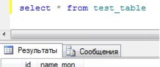
SELECT LASTNAME, FIRSTNAME from PERSON WHERE AGE \u003d 28
If we have an index on the age column, then the optimizer will use the index to find all 28-year-olds and then query the IDs of the corresponding table rows, since the index only contains age information.Let's say we have a different request:
SELECT TYPE_PERSON.CATEGORY from PERSON, TYPE_PERSON WHERE PERSON.AGE \u003d TYPE_PERSON.AGE
For joining with TYPE_PERSON, the index on the PERSON column will be used. But since we did not request information from the PERSON table, no one will access it by row IDs.This approach is only good for a small number of hits because it is expensive in terms of I / O. If you need to frequently contact by ID, it is better to use full scan.
- other methods... You can read about them in the Oracle documentation. Different databases may use different names, but the principles are the same everywhere.
So, we know how to get the data, it's time to merge them. But first, let's define some new terms: internal dependencies and external dependencies... The addiction can be:
- table,
- index,
- an intermediate result of a previous operation (for example, a previous join).
Most often, the cost of A JOIN B is not equal to the cost of B JOIN A.
Suppose the outer dependency contains N elements and the inner one contains M. As you remember, the optimizer knows these values \u200b\u200bthrough statistics. N and M are the cardinal numbers of the dependencies.
- Union using nested loops. This is the simplest way to combine.

It works like this: for each line of the external dependency, matches are searched for all lines of the internal dependency.
Example pseudocode:
Nested_loop_join (array outer, array inner) for each row a in outer for each row b in inner if (match_join_condition (a, b)) write_result_in_output (a, b) end if end for end for
Since this is a double iteration, the time complexity is O (N * M).For each of the N lines of the external dependence, M lines of the external dependence must be counted. That is, this algorithm requires N + N * M disk reads. If the internal dependence is small enough, then you can put it entirely in memory, and then the disk subsystem will only have M + N reads. So it is recommended to make the internal dependency as compact as possible in order to drive it into memory.
In terms of time complexity, there is no difference.
It is also possible to replace the internal dependency with an index, which will save I / O operations.
If the internal dependency does not fit into memory entirely, you can use a different algorithm that uses disk more economically.- Instead of reading both dependencies line by line, they are read in groups of lines (bunch), with one group from each dependency stored in memory.
- Lines from these groups are compared with each other, and the found matches are saved separately.
- Then new groups are loaded into memory and are also compared with each other.
Algorithm example:
// improved version to reduce the disk I / O. nested_loop_join_v2 (file outer, file inner) for each bunch ba in outer // ba is now in memory for each bunch bb in inner // bb is now in memory for each row a in ba for each row b in bb if (match_join_condition ( a, b)) write_result_in_output (a, b) end if end for end for end for end for
In this case, the time complexity remains the same, but the number of disk accesses decreases: (the number of external groups + the number of external groups * the number of internal groups). As the group size grows, the number of disk accesses decreases even more.Note: in this algorithm, more data is read on each call, but this does not matter, since the calls are sequential.
- Hash join. This is a more complex operation, but in many cases the cost is lower.

The algorithm is as follows:
- All elements from the internal dependency are read.
- A hash table is created in memory.
- All elements from the external dependency are read one by one.
- For each item, a hash is calculated (using the appropriate function from the hash table) so that the corresponding block in the internal dependency can be found.
- Items from the block are compared to items from the external dependency.
- An internal dependency contains X blocks.
- The hash function distributes hashes almost the same for both dependencies. That is, all blocks are of the same size.
- The cost of finding a match between elements of an external dependency and all elements within a block is equal to the number of elements within a block.
(M / X) * (N / X) + hashtable_cost (M) + hash_cost * N
And if the hash function creates small enough blocks, then the time complexity will be O (M + N).
There is another hash join method that is more memory efficient and does not require more I / O:
- Hash tables are computed for both dependencies.
- Placed on disk.
- And then they are compared behaviorally with each other (one block is loaded into memory, and the second is read line by line).
The union operation can be divided into two stages:
- (Optional) A sort join is performed first, when both input datasets are sorted by the join keys.
- Then the merge takes place.
The merge sort algorithm has already been discussed above, in this case it is quite justified if it is important for you to save memory.
But it happens that datasets come already sorted, for example:
- If the table is organized natively.
- If the dependency is an index when a join condition is present.
- If the union occurs with an intermediate sorted result.

This operation is very similar to the merge operation in the merge sort procedure. But instead of selecting all members of both dependencies, we only select equal members.
- The two current members of both dependencies are compared.
- If they are equal, then they are entered into the resulting table, and then the next two elements are compared, one from each dependency.
- If they are not equal, then the comparison is repeated, but instead of the smallest of the two elements, the next element from the same dependence is taken, since the probability of coincidence in this case is higher.
- Steps 1-3 are repeated until you run out of elements of one of the dependencies.
If both dependencies still need to be sorted, then the time complexity is O (N * Log (N) + M * Log (M)).
This algorithm works well because both dependencies are already sorted and we don't have to traverse them back and forth. However, some simplification is allowed here: the algorithm does not handle situations when the same data occurs multiple times, that is, when multiple matches occur. In reality, a more complex version of the algorithm is used. For instance:
MergeJoin (relation a, relation b) relation output integer a_key: \u003d 0; integer b_key: \u003d 0; while (a! \u003d null and b! \u003d null) if (a< b) a_key++; else if (a > b) b_key ++; else // Join predicate satisfied write_result_in_output (a, b) // We need to be careful when we increase the pointers integer a_key_temp: \u003d a_key; integer b_key_temp: \u003d b_key; if (a! \u003d b) b_key_temp: \u003d b_key + 1; end if if (b! \u003d a) a_key_temp: \u003d a_key + 1; end if if (b \u003d\u003d a && b \u003d\u003d a) a_key_temp: \u003d a_key + 1; b_key_temp: \u003d b_key + 1; end if a_key: \u003d a_key_temp; b_key: \u003d b_key_temp; end if end while
If there was a better way to combine, then all these varieties would not exist. So the answer to this question depends on a bunch of factors:
- Available memory... If it's not enough, forget about powerful hash join. At least, about its implementation entirely in memory.
- The size of the two test cases. If you have one table large and the other very small, then a nested loop join will work the fastest, because hash joins are expensive to create hashes. If you have two very large tables, then nested loop joins will consume all the CPU resources.
- Availability of indices. If you have two B-tree indexes, it is better to use merge join.
- Whether the result needs to be sorted. You might want to use an expensive merge (sorted) join if you are working with unsorted datasets. Then the output will be sorted data, which is more convenient to combine with the results of another merge. Or because the query, implicitly or explicitly, involves getting data sorted by the ORDER BY / GROUP BY / DISTINCT statements.
- Are output dependencies sorted... In this case, it is better to use merge join.
- What types of dependencies are you using... Equivalence join (table.column1 \u003d table.B.column2)? Internal dependencies, external, cartesian product or self-join? In different situations, some combination methods do not work.
- Data distribution... If the data is rejected based on a join condition (for example, you unite people by last name, but there are often namesakes), then in no case should you use hash join. Otherwise, the hash function will create buckets with a very poor internal distribution.
- Whether it is necessary to merge into multiple processes / threads.
4.4.4. Simplified examples
Let's say we need to combine five tables to get a complete picture of some people. Everyone can have:
- Several mobile phone numbers.
- Multiple email addresses.
- Several physical addresses.
- Several bank account numbers.
SELECT * from PERSON, MOBILES, MAILS, ADRESSES, BANK_ACCOUNTS WHERE PERSON.PERSON_ID \u003d MOBILES.PERSON_ID AND PERSON.PERSON_ID \u003d MAILS.PERSON_ID AND PERSON.PERSON_ID \u003d ADRESSES.PERSON_ID AND PERSON_ID \u003d ADRESSES.PERSON_ID AND PERSON_ID
The optimizer needs to find the best way to process the data. But there are two problems:
- Which way to combine to use? There are three options (hash join, merge join, nested loop join), with the option to use 0, 1, or 2 indices. Not to mention, the indexes can be different too.
- In what order should you merge?

Based on the above, what options are there?
- Use a brute-force approach. Using statistics, calculate the cost of each of the possible query execution plans and choose the cheapest one. But there are quite a few options. For each join order, three different join methods can be used, for a total of 34 \u003d 81 possible execution plans. In the case of a binary tree, the problem of choosing the join order turns into a permutation problem, and the number of options is (2 * 4)! / (4 + 1)! .. As a result, in this very simplified example, the total number of possible query execution plans is 34 * (2 * 4)! / (4 + 1)! \u003d 27 216. If we add to this the options where 0, 1 or 2 B-tree indexes are used in a merge join, the number of possible plans rises to 210,000. Did we mention that this is a VERY SIMPLE query?
- Cry and quit. Very tempting, but unproductive, and money is needed.
- Try several plans and choose the cheapest one. Since it is impossible to calculate the cost of all possible options, you can take an arbitrary test dataset and run all types of plans over it in order to estimate their cost and choose the best one.
- Apply smart rules to reduce the number of possible plans.
There are two types of rules:- "Logical", with which you can exclude useless options. But they are far from always applicable. For example, "when joining with nested loops, the inner dependency should be the smallest dataset."
- You can avoid looking for the most profitable solution and apply more stringent rules to reduce the number of possible plans. Say, "if the dependency is small, use a nested loop join, but never a merge join or hash join."
So how does the database make choices?
4.4.5. Dynamic programming, greedy algorithm and heuristics
A relational database uses different approaches, which were mentioned above. And the job of the optimizer is to find a suitable solution within a limited time. In most cases, the optimizer is not looking for the best, but simply the good solution.
Brute force can be suitable for small requests. And with ways to eliminate unnecessary computation, brute force can be used even for medium-sized queries. This is called dynamic programming.
Its essence lies in the fact that many execution plans are very similar.

In this illustration, all four plans use the subtree A JOIN B. Instead of calculating its cost for each plan, we can only count it once and then use that data as much as necessary. In other words, with the help of memoization, we solve the overlap problem, that is, we avoid unnecessary calculations.
Thanks to this approach, instead of the time complexity (2 * N)! / (N + 1)! we get "only" 3 N. As applied to the previous example with four joins, this means reducing the number of options from 336 to 81. If we take a query with 8 joins (a small query), the complexity will decrease from 57,657,600 to 6,561.
If you are already familiar with dynamic programming or algorithms, you can play around with this algorithm:
Procedure findbestplan (S) if (bestplan [S] .cost infinite) return bestplan [S] // else bestplan [S] has not been computed earlier, compute it now if (S contains only 1 relation) set bestplan [S]. plan and bestplan [S] .cost based on the best way of accessing S / * Using selections on S and indices on S * / else for each non-empty subset S1 of S such that S1! \u003d S P1 \u003d findbestplan (S1) P2 \u003d findbestplan (S - S1) A \u003d best algorithm for joining results of P1 and P2 cost \u003d P1.cost + P2.cost + cost of A if cost< bestplan[S].cost
bestplan[S].cost = cost
bestplan[S].plan = “execute P1.plan; execute P2.plan;
join results of P1 and P2 using A”
return bestplan[S]
Dynamic programming can be used for larger queries, but additional rules (heuristics) have to be introduced to reduce the number of possible plans: 
Greedy algorithms
But if the request is very large, or if we need to get an answer extremely quickly, another class of algorithms is used - greedy algorithms.
In this case, a query execution plan is built step by step using a certain rule (heuristic). Thanks to it, the greedy algorithm looks for the best solution for each stage separately. The plan starts with a JOIN statement, and then a new JOIN is added at each stage according to the rule.
Let's look at a simple example. Let's take a query with 4 joins of 5 tables (A, B, C, D and E). Let's simplify the task a little and imagine that the only option is to combine using nested algorithms. We will use the rule “apply least cost join”.
- We start with one of the tables, for example A.
- We calculate the cost of each union with A (it will be both in the role of external and internal dependence).
- We find that A JOIN B will cost us the least.
- Then we calculate the cost of each union with the result A JOIN B (we also consider it in two roles).
- We find that the most profitable is (A JOIN B) JOIN C.
- Again, we assess the possible options.
- At the end, we get the following query execution plan: (((A JOIN B) JOIN C) JOIN D) JOIN E) /
This algorithm is called the "Nearest Neighbor Algorithm".
We will not go into details, but with good modeling of the complexity of the N * log (N) sorting, this problem can be. The time complexity of the algorithm is O (N * log (N)) instead of O (3 N) for the full version with dynamic programming. If you have a large query with 20 joins, that would be 26 versus 3 486 784 401. A big difference, right?
But there is a nuance. We assume that if we can find the best way to join the two tables, we will get the lowest cost when the result of the previous joins is combined with the following tables. However, even if A JOIN B is the cheapest option, then (A JOIN C) JOIN B may have a lower cost than (A JOIN B) JOIN C.
So if you desperately need to find the cheapest plan of all time, then we can advise you to run greedy algorithms repeatedly using different rules.
Other algorithms
If you are already fed up with all these algorithms, then you can skip this chapter. It is not necessary to master the rest of the material.
Many researchers deal with the problem of finding the best query execution plan. They often try to find solutions for specific tasks and patterns. For example, for star joins, parallel query execution, etc.
We are looking for alternatives to replace dynamic programming for the execution of large queries. The same greedy algorithms are a subset of heuristic algorithms. They act according to the rule, remember the result of one stage and use it to find the best option for the next stage. And algorithms that do not always use the solution found for the previous stage are called heuristic.
An example is genetic algorithms:
- Each solution is a plan for the full execution of the request.
- Instead of one solution (plan), the algorithm generates X solutions at each stage.
- First, X plans are created, this is done randomly.
- Of these, only those plans are saved whose cost satisfies a certain criterion.
- These plans are then mixed to create X new plans.
- Some of the new plans are randomly modified.
- The previous three steps are repeated Y times.
- From the plans of the last cycle we get the best one.
By the way, genetic algorithms are integrated into PostgreSQL.
The database also uses such heuristic algorithms as Simulated Annealing, Iterative Improvement, Two-Phase Optimization. But it is not a fact that they are used in corporate systems, perhaps their destiny is research products.
4.4.6. Real optimizers
Also an optional chapter, you can skip it.
Let's move away from theorizing and look at real-life examples. For example, how the SQLite optimizer works. It is a "lightweight" database using a simple greedy optimization with additional rules:
- SQLite never changes the order of tables in a CROSS JOIN operation.
- It uses nested loops union.
- Outside joins are always evaluated in the order in which they occurred.
- Up to version 3.8.0, the greedy Nearest Neighor algorithm is used to find the best query execution plan. And since version 3.8.0 “N Nearest Neighbors” (N3, N Nearest Neighbors) is applied.
- Greedy Algorithms:
- 0 - minimal optimization. Uses index scans, nested loops joins, and avoids rewriting some queries.
- 1 - low optimization
- 2 - full optimization
- Dynamic programming:
- 3 - medium optimization and rough approximation
- 5 - full optimization, all heuristic techniques are used
- 7 - the same, but without the heuristic
- 9 - maximum optimization at any cost, regardless of the effort expended. All possible ways of combining are evaluated, including Cartesian products.
- Collect all possible statistics, including frequency distributions and quantiles.
- Applying all query rewrite rules, including composing a table route for materialized queries). The exception is computationally intensive rules that are used in a very limited number of cases.
- When iterating over the join options using dynamic programming:
- Composite internal dependency is used to a limited extent.
- For star charts with conversion tables, Cartesian products are limited.
- A wide range of access methods are covered, including list prefetching (more on that below), special AND index operations, and table-routing for materialized queries.
Other conditions (GROUP BY, DISTINCT, etc.) are handled by simple rules.
4.4.7. Query plan cache
Because planning takes time, most databases store the plan in the query plan cache. This helps to avoid unnecessary computation of the same steps. The database needs to know exactly when it needs to update outdated plans. For this, a certain threshold is set, and if changes in statistics exceed it, the plan related to this table is removed from the cache.
Executor of requests
At this stage, our plan has already been optimized. It is recompiled into executable code and, if resources are sufficient, it is executed. The statements contained in the plan (JOIN, SORT BY, etc.) can be processed both sequentially and in parallel, the decision is made by the executor. To receive and write data, it interacts with the data manager.5. Data manager

The query manager is executing a query and needs data from tables and indexes. He requests them from the data manager, but there are two difficulties:
- Relational databases use a transactional model. It is impossible to get any desired data at a specific point in time, because at this time they can be used / modified by someone.
- Retrieving data is the slowest operation in the database. Therefore, the data manager needs to be able to predict its work in order to fill the memory buffer in a timely manner.
5.1. Cache manager
As has been said more than once, the bottleneck in the database is the disk subsystem. Therefore, a cache manager is used to improve performance.
Instead of receiving data directly from the file system, the query executor turns to the cache manager for it. It uses the buffer pool contained in memory, which can dramatically increase the performance of the database. This is difficult to estimate in numbers, since a lot depends on what you need:
- Sequential access (full scan) or random (access by line ID).
- Read or write.
However, here we are faced with another problem. The cache manager needs to put data in memory BEFORE the query executor needs it. Otherwise, it will have to wait for them to be received from the slow disk.
5.1.1. Proactive
The executor of requests knows what data he will need, since he knows the whole plan, what data is contained on the disk and statistics.
When the executor processes the first chunk of data, it asks the cache manager to preload the next chunk. And when it proceeds to processing it, it asks the DC to load the third one and confirms that the first portion can be removed from the cache.
The cache manager stores this data in a buffer pool. It also adds service information (trigger, latch) to them to know if they are still needed in the buffer.
Sometimes the executor does not know what data he will need, or some databases do not have such functionality. Then speculative prefetching is used (for example, if the executor requests data 1, 3, 5, it will probably request 7, 9, 11 in the future) or sequential prefetching (in this case, the DC simply loads the next order a piece of data.
Remember, the buffer is limited by the amount of available memory. That is, to load some data, we have to periodically delete others. Filling and flushing the cache consumes some disk and network resources. If you have a frequently executed query, it would be counterproductive to load and clear the data it uses every time. To solve this problem, modern databases use a buffer replacement strategy.
5.1.2. Buffer swap strategies
Most databases (at least SQL Server, MySQL, Oracle and DB2) use the LRU (Least Recently Used) algorithm for this. It is designed to keep the data in the cache that was recently used, which means it is highly likely that it may be needed again.

To make it easier to understand the operation of the algorithm, let us assume that the data in the buffer is not blocked by triggers (latch), and therefore can be deleted. In our example, the buffer can store three chunks of data:
- The cache manager uses data 1 and puts it in an empty buffer.
- Then it uses data 4 and sends it to the buffer too.
- The same is done with data 3.
- Further data is taken 9. But the buffer is already full. Therefore, data 1 is deleted from it, since it has not been used for the longest time. After that, data 9 is placed in the buffer.
- The cache manager is using data 4 again. It is already in the buffer, so it is marked as last used.
- Data 1 is again in demand. To put it in the buffer, data 3 is deleted from it, as it has not been used the longest.
Algorithm improvements
To prevent this from happening, some databases use special rules. According to Oracle documentation:
“For very large tables, direct access is usually used, that is, blocks of data are read directly to avoid a cache buffer overflow. For medium-sized tables, both direct access and read from the cache can be used. If the system decides to use the cache, then the database puts the data blocks at the end of the LRU list to prevent flushing the buffer. "
An improved version of LRU - LRU-K is also used. SQL Server uses LRU-K when K \u003d 2. The essence of this algorithm is that when assessing a situation, it takes into account more information about past operations, and not only remembers the last used data. The letter K in the name means that the algorithm takes into account which data was used the last K times. They are assigned a certain weight. When new data is loaded into the cache, the old, but often used data are not deleted, because their weight is higher. Of course, if the data is no longer used, it will still be deleted. And the longer the data remains unclaimed, the more its weight decreases over time.
Calculating the weight is quite expensive, so SQL Server uses LRU-K when K is only 2. With some increase in the value of K, the efficiency of the algorithm improves. You can get to know him better thanks to.
Other algorithms
Of course, LRU-K is not the only solution. There are also 2Q and CLOCK (both are similar to LRU-K), MRU (Most Recently Used, which uses LRU logic, but a different rule applies, LRFU (Least Recently and Frequently Used), etc. In some databases, you can choose, what algorithm will be used.
5.1.3. Write buffer
We talked only about the read buffer, but DBs also use write buffers, which accumulate data and flush it to disk in portions, instead of sequential writes. This saves I / O operations.
Remember that buffers store pages (indivisible data units), not rows from tables. A page in the buffer pool is called dirty if it has been modified but not written to disk. There are many different algorithms by which the timing of dirty page writes is selected. But this has a lot to do with the notion of transactions.
5.2. Transaction manager
His job is to make sure that each request is executed with its own transaction. But before we talk about the dispatcher, let's clarify the concept of ACID transactions.5.2.1. "Under acid" (a play on words, if someone does not understand)
An ACID transaction (Atomicity, Isolation, Durability, Consistency) is an elementary operation, a unit of work that satisfies 4 conditions:
- Atomicity There is nothing "less" than a transaction, no more minor transaction. Even if the transaction lasts 10 hours. If the transaction fails, the system returns to the "before" state, that is, the transaction is rolled back.
- Isolation... If two transactions A and B are executed at the same time, then their result should not depend on whether one of them completed before, during or after the execution of the other.
- Durability. When a transaction is committed (commited), that is, successfully completed, the data used by it remains in the database, regardless of possible incidents (errors, crashes).
- Consistency (consistency). Only valid data is written to the database (in terms of relational and functional relationships). Consistency depends on atomicity and isolation.

During the execution of a transaction, you can execute various SQL queries for reading, creating, updating and deleting data. Problems start when two transactions use the same data. A classic example is the transfer of money from account A to account B. Let's say we have two transactions:
- T1 takes $ 100 from account A and sends it to account B.
- T2 takes $ 50 from account A and sends it to account B.
- Atomicity allows you to be sure that no matter what event occurs during T1 (server crash, network failure), it cannot happen that $ 100 will be debited from A, but will not come to B (otherwise they speak of an "inconsistent state").
- Isolation says that even if T1 and T2 are carried out simultaneously, as a result, $ 100 will be written off from A and the same amount will go to B. In all other cases, they again speak of an inconsistent state.
- Reliability allows you not to worry about T1 disappearing if the base falls immediately after the T1 commit.
- Consistency prevents the possibility of money being created or destroyed in the system.
Many databases do not provide complete isolation by default, as this leads to huge performance overhead. SQL uses 4 levels of isolation:
- Serializable transactions. Highest level of isolation. The default is used in SQLite. Each transaction runs in its own fully isolated environment.
- Repeatable read. Used by MySQL by default. Each transaction has its own environment, with the exception of one situation: if the transaction adds new data and succeeds, they will be visible to other transactions still in progress. But if the transaction modifies data and succeeds, these changes will not be visible to transactions that are still in progress. That is, the principle of isolation is violated for new data.
For example, transaction A performs
SELECT count (1) from TABLE_X
Then transaction B adds to table X and commits new data. And if after that transaction A again executes count (1), then the result will be different.This is called phantom reading.
- Read commited... Used by default in Oracle, PostgreSQL and SQL Server. This is the same as repeated read, but with an additional isolation violation. Let's say transaction A reads data; they are then modified or deleted by transaction B, which commits these actions. If A again reads this data, then she will see the changes (or the fact of deletion) made by B.
This is called a non-repeatable read.
- Read uncommited data. Lowest level of isolation. A new isolation violation is added to the read committed data. Let's say transaction A reads data; they are then modified by transaction B (changes are not committed, B is still in progress). If A reads the data again, it will see the changes made. If B is pumped back, then upon repeated reading A will not see any changes, as if nothing had happened.
This is called dirty reading.
Most databases add their own isolation levels (for example, based on snapshots, as in PostgreSQL, Oracle and SQL Server). Also, many databases do not implement all four of the above levels, especially reading uncommitted data.
A user or developer can override the default isolation level immediately after establishing a connection. To do this, just add a very simple line of code.
5.2.2. Concurrency control
The main thing for which we need isolation, consistency and atomicity is the ability to perform write operations on the same data (add, update and delete).
If all transactions read data only, they can work simultaneously without affecting other transactions.
If at least one transaction changes the data read by other transactions, then the database needs to find a way to hide these changes from them. You also need to make sure that the changes made will not be deleted by other transactions that do not see the changed data.
This is called concurrency control.
The easiest way is to simply execute transactions one at a time. But this approach is usually ineffective (only one core of one processor is used), and it also loses the scalability.
The ideal way to solve the problem looks like this (every time a transaction is created or canceled):
- Monitor all operations of each transaction.
- If two or more transactions conflict due to reading / modifying the same data, then change the order of operations within the parties to the conflict in order to minimize the number of reasons.
- Execute conflicting parts of transactions in a specific order. Non-conflicting transactions are executed in parallel at this time.
- Keep in mind that transactions can be canceled.
5.2.3. Lock manager
To solve the above problem, many databases use locks and / or data versioning.
If a transaction needs some data, then it blocks it. If another transaction also required them, then it will have to wait until the first transaction releases the lock.
This is called exclusive blocking.
But it is too wasteful to use exclusive locks when transactions only need to read data. Why interfere with reading data? In such cases, shared locks are used. If a transaction needs to read data, it applies a shared lock and reads it. This does not prevent other transactions from sharing locks and reading data too. If any of them needs to change the data, then it will have to wait until all shared locks are removed. Only then can she apply an exclusive lock. And then all other transactions will have to wait for its removal in order to read this data.

A lock manager is a process that applies and releases locks. They are stored in a hash table (the keys are the data being locked). The dispatcher knows for all data which transactions have applied locks or are waiting to release them.
Deadlock
Using locks can lead to a situation where two transactions are waiting indefinitely to release locks:

Here, transaction A has exclusively locked data 1 and is awaiting the release of data 2. At the same time, transaction B has exclusively locked data 2 and is waiting for the release of data 1.
In a deadlock, the dispatcher chooses which transaction to cancel (rollback). And the decision is not so easy to make:
- Would it be better to kill the transaction that changed the last dataset (which means rollback will be the least painful)?
- Would it be better to kill the youngest transaction since users of other transactions have waited longer?
- Would it be better to kill a transaction that takes less time to complete?
- How many other transactions will the rollback affect?
Let's imagine a hash table in the form of a diagram, as in the illustration above. If a cyclic link is present in the diagram, the interlock is confirmed. But since it is expensive to check for loops (after all, the diagram on which all locks are reflected will be quite large), a simpler approach is often used: using timeouts. If the lock is not released within a certain amount of time, then the transaction has entered a deadlock state.
The dispatcher can also check to see if it will cause a deadlock before locking. But to answer this unambiguously, you also have to spend money on calculations. Therefore, such pre-checks are often presented as a set of basic rules.
Two-phase blocking
Complete isolation is most easily achieved when the lock is applied at the beginning and released at the end of the transaction. This means that a transaction has to wait until all locks are released before starting, and the locks it has applied are released only after completion. This approach can be used, but then a lot of time is wasted on all these waiting for the release of locks.
DB2 and SQL Server use the two-phase locking protocol, which divides a transaction into two phases:
- The growing phasewhen a transaction can only apply locks, but not release them.
- Shrinking phasewhen a transaction can only release locks (from data that has already been processed and will not be processed again), but not apply new ones.

Before transaction A, X \u003d 1 and Y \u003d 1. It processes data Y \u003d 1, which was changed by transaction B after the beginning of transaction A. Due to the principle of isolation, transaction A must process Y \u003d 2.
Objectives to be met using these two simple rules:
- Release locks that are no longer needed to reduce the waiting time for other transactions.
- Prevent cases where a transaction receives data modified by a previously started transaction. Such data does not match the requested one.
Of course, real databases use more complex systems, more types of locks and with greater granularity (locks for rows, pages, partitions, tables, table spaces), but the essence is the same.
Data versioning
Another way to solve the problem of transaction conflict is to use data versioning.
- All transactions can update the same data at the same time.
- Each transaction works with its own copy (version) of the data.
- If two transactions change the same data, then only one of the modifications is accepted, the other will be rejected, and the transaction that made it will be rolled back (and possibly restarted).
- Read transactions do not block write transactions, and vice versa.
- The clumsy lock manager has no effect.
Both locks and versioning approaches have pros and cons, much depends on the situation in which they are applied (more reads or more writes). You can check out a very good presentation on implementing multiversion concurrency control in PostgreSQL.
Some databases (DB2 prior to version 9.7, SQL Server) use only locks. Others, like PostgreSQL, MySQL, and Oracle, use a combination of approaches.
Note: Versioning has an interesting effect on indexes. Sometimes duplicates appear in a unique index, the index may contain more records than rows in the table, etc.
If part of the data is read at one level of isolation, and then it increases, then the number of locks increases, which means more time is wasted waiting for transactions. Therefore, most databases do not use the maximum isolation level by default.
As usual, refer to the documentation for more details: MySQL, PostgreSQL, Oracle.
5.2.4. Log manager
As we already know, for the sake of increasing performance, the database stores part of the data in the buffer memory. But if the server crashes while committing a transaction, the data in memory will be lost. And this violates the principle of the reliability of transactions.
Of course, you can write everything to disk, but if you crash, you will be left with incomplete data, and this is already a violation of the atomicity principle.
Any changes written by the transaction must be rolled back or completed.
This is done in two ways:
- Shadow Copies / Pages. Each transaction creates its own copy of the database (or part of it), and works with this copy. If an error occurs, the copy is deleted. If everything went well, then the database instantly switches to the data from the copy using one trick at the file system level, and then deletes the "old" data.
- Transaction log. This is a special storage. Before each writing to the disk, the database writes information to the transaction log. So in the event of a crash, the database will know how to delete or complete the unfinished transaction.
In large databases with numerous transactions, shadow copies / pages take up an incredible amount of disk space. Therefore, modern databases use the transaction log. It should be located in a fault-free storage.
Most products (in particular, Oracle, SQL Server, DB2, PostgreSQL, MySQL and SQLite) work with transaction logs via WAL (Write-Ahead Logging) protocol. This protocol contains three rules:
- Each modification to the database must be accompanied by a log entry, and it must be entered BEFORE the data is written to disk.
- Log entries should be arranged in accordance with the order of the corresponding events.
- When a transaction is committed, a record of this must be logged BEFORE the successful completion of the transaction.

The implementation of these rules is monitored by a log manager. It sits logically between the cache manager and the data access manager. The log manager logs every operation performed by transactions until it is written to disk. Seems right?
WRONG! After everything we've been through in this article, it's time to remember that everything related to the database is subject to the curse of the "database effect". Seriously, the problem is finding a way to write to the log while maintaining good performance. After all, if the transaction log is slow, then it slows down all other processes.
ARIES
In 1992, researchers at IBM created an extended version of WAL called ARIES. ARIES is used in one form or another by most modern databases. If you want to study this protocol more deeply, you can study the corresponding work.
So ARIES stands for Algorithms for Recovery and Isolation Exploiting Semantics. This technology has two objectives:
- Provide good performance when writing logs.
- Provide fast and reliable recovery.
- The user canceled it.
- Server or network error.
- The transaction violated the integrity of the database. For example, you applied the UNIQUE clause to a column and the transaction added a duplicate.
- The presence of deadlocks.
How is this possible? To answer this, you first need to figure out what information is stored in the log.
Logs
Each operation (add / delete / change) during the execution of a transaction leads to the appearance of a record in the log. The record contains:
- LSN (Log Sequence Number)... This is a unique number, the meaning of which is determined in chronological order. That is, if operation A occurred before operation B, the LSN for A will be less than the LSN for B. In reality, the method for generating the LSN is more complicated, since it is also related to the way the log is stored.
- TransID. ID of the transaction that performed the operation.
- PageID... Disk space where modified data is located.
- PrevLSN... Link to a previous log entry created by the same transaction.
- UNDO... How to rollback an operation.
For example, if an update operation was performed, then the previous value / state of the changed element (physical UNDO) or the reverse operation is written to UNDO, allowing you to return to the previous state (logical UNDO). ARIES uses only logical, physical work is very difficult.
- REDO... Method of repeating the operation.
As far as is known, UNDO is not only used in PostgreSQL. Instead, a garbage collector is used to clean up old versions of the data. This is due to the implementation of data versioning in this DBMS.
To make it easier for you to imagine the composition of the log entry, here is a visual simplified example in which the UPDATE FROM PERSON SET AGE \u003d 18; query is executed. Let it be executed in transaction number 18:

Each log has a unique LSN. Linked logs refer to the same transaction, and they are linked in chronological order (the last log in the list refers to the last operation).
Log buffer
To prevent logging from becoming a bottleneck in the system, a log buffer is used.

When the query executor requests the modified data:
- The cache manager stores them in a buffer.
- The log manager stores the corresponding log in its own buffer.
- The executor of the requests determines whether the operation has completed and, accordingly, whether the changed data can be requested.
- The log manager stores the necessary information in the transaction log. The moment of making this record is set by the algorithm.
- The cache manager writes the changes to disk. The moment of recording is also set by the algorithm.
STEAL and FORCE policies
To improve performance, step 5 should be done after the commit, since in the event of a failure it is still possible to restore the transaction using REDO. This is called the "NO-FORCE policy".
But the database can also choose the FORCE policy to reduce the load during recovery. Then step number 5 is executed before commit.
The database also chooses whether to write data to disk step by step (STEAL policy) or, if the buffer manager must wait for the commit, write everything at once (NO-STEAL). The choice depends on what you want: fast recording with long recovery or fast recovery?
How the mentioned policies affect the recovery process:
- STEAL / NO-FORCE requires UNDO and REDO. Performance is superior, but more complex structure of logs and recovery processes (like ARES). Most databases use this combination of policies.
- STEAL / FORCE only needs UNDO.
- For NO-STEAL / NO-FORCE - only REDO.
- For NO-STEAL / FORCE, nothing is needed at all. Performance in this case is the lowest, and a huge amount of memory is required.
So how can we use our wonderful logs? Suppose a new employee crashes the database (rule # 1: the newbie is always to blame!). You restart it and the recovery process begins.
ARIES rebuilds in three steps:
- Analysis... The entire transaction log is read so that the chronology of events that occurred during the base fall can be restored. This helps determine which transaction to roll back. All transactions are rolled back without a commit order. The system also decides what data should have been written to disk during the crash.
- Repeat... REDO is used to update the database to the state before the crash. Its logs are processed in chronological order. For each log, the LSN of the page on disk containing the data to be changed is read.
If LSN (pages_on_disk)\u003e \u003d LSN (records_in_log), then data has already been written to disk before the crash. But the value was overwritten by an operation that was performed after writing to the log and before the failure. So nothing has really been done.
If LSN (pages_on_disk)
Rollback is performed even for transactions that will be rolled back because it simplifies the recovery process. But modern databases probably don't.
- Cancel. At this stage, all transactions that were not completed at the time of the failure are rolled back. The process starts with the last logs of each transaction and processes the UNDO in reverse chronological order using PrevLSN.
If the transaction is canceled “manually”, either by the lock manager, or due to a network failure, then the analysis step is not needed. After all, information for REDO and UNDO is contained in two tables located in memory:
- In the transactions table (the states of all current transactions are stored here).
- The dirty page table (contains information about what data needs to be written to disk).
The analysis stage is needed just to restore both tables using information from the transaction log. ARIES uses checkpoints to expedite this phase. The contents of both tables are written to disk from time to time, as well as the last one at the time of the LSN recording. So during recovery, only the logs following this LSN are analyzed.
6. Conclusion
As an additional overview reading about databases, I recommend the article Architecture of a Database System. This is a good introduction to the topic, written in a fairly straightforward language.If you have carefully read all of the above material, then you probably got an idea of \u200b\u200bhow great the capabilities of databases are. However, this article does not cover other important issues:
- How to manage clustered databases and global transactions.
- How to get a snapshot if the database is working.
- How to store and compress data efficiently.
- How to manage memory.
So, if someone asks you, how do databases work, then instead of spitting and leaving, you can answer:

Tags: Add Tags