This stuff has an answer on how to freeze a string in excel. We will see how to freeze the first (top) or arbitrary row, as well as how to freeze an area in excel.
Freezing a row or column in Excel is an extremely useful feature, especially for creating lists and tables with a large amount of data arranged in cells and columns. By pinning a row, you can easily track the headings of certain columns, which means you save time instead of endlessly scrolling up and down.
Let's look at an example. In the image below, we see the first row, which is the column headings.
Agree, it will be inconvenient for us to enter and read data from the table if we do not know or see the headers at the top. Therefore, we will fix the upper term in excel as follows. In the upper menu of Excel, we find the item "VIEW", in the submenu that opens, select "FIX AREAS", and then select the sub-item "FIX TOP ROW".

These simple actions to freeze a line allow you to scroll through the document and at the same time understand the meaning of the row headers in Excel. I repeat - this is convenient when there are a large number of lines.

I must say that the same effect can be achieved if you first select the cells of the entire first row, and then apply the first sub-item of the already known submenu "FIX AREAS" - "Freeze Areas":

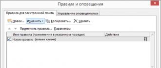
Well, now about how to freeze a region in excel. First, select the area of \u200b\u200bthe Excel cells that you want to constantly see (fix). It can be several lines and an arbitrary number of cells. As you probably already guessed, the path to this pinning function remains the same: the menu item "VIEW" → then "PINCH AREAS" → then the sub-item "PINCH AREAS". The upper figure illustrates this.
If for some reason you could not correctly freeze rows or areas in excel, go to the menu "VIEW" → "PINCH AREAS" → select "Unpin areas". Now you can try again slowly to capture the desired lines and areas of the document.
Finally, I will say that the first column also lends itself to fixing. We also act → menu "VIEW" → "ANCHOR AREAS" → select the item "Anchor first column".

Good luck with working with documents in Excel, make no mistakes and save your time using the additional functions and tools of this editor.
Excel program is used not only for calculations, creating tables, graphing. It also allows you to conveniently view large tables, thanks to the ability to pin the table header, which will always stay in place when you scroll the table. In this article, we will take a look at how to freeze a region in Excel, which will freeze not only the top rows, but also the columns to the left, or both columns and rows.
When looking through large multi-page tables, it is very difficult to navigate when the table header is not visible. You can dock a region in Excel 2010 through the View tab menu. In the "Window" sector there is an item "Freeze Areas", by clicking on which we are given three options. Let's consider each of them in more detail.
 Menu \\ "Freeze Areas \\" in Excel
First, let's take a look at how to freeze the top row in Excel. We need to determine how many lines we need to freeze and place the cursor on the line below, i.e. if you need to fix the header of the table, you must select any cell with data right under the header, and then apply the menu item "Fix the top row". Now, when scrolling the sheet, the selected table header will always be at the top.
 The result of applying the item \\ "Fix the upper drain \\" in Excel
Now let's look at how to freeze the first column in Excel. In this case, it is no longer necessary to select the required cell, since by applying the item "Freeze the first column" in any case, only the first column in Excel will be fixed.
 The result of applying the item \\ "Freeze first column \\" in Excel
There is one more menu item that will allow you to freeze an area in Excel that is much larger than a few rows at the top or the first column. The item "Freeze regions" allows you to freeze several rows at the top and several columns to the left. Before using it, you need to select a cell that will be the intersection of the docked areas, i.e. the rows at the top and columns to the left of the cell are frozen.
 The result of applying the item \\ "Freeze areas \\" in Excel
After pinning any area, a new item "Unpinned Areas" appears in the menu, after which all pinned areas will be unlocked.
Today we will talk about how to freeze columns in Excel. When working with various tabular data, it is often necessary to see the headings of rows or columns in front of you, throughout the entire process, at every moment in time, regardless of the given position of the scroll pointer. Fortunately, the specified application has a special function that can help us.
Preparation
In order to solve the question of how to fix columns and rows in Excel, start the spreadsheet editor and open a file with the necessary data in it. Next, go to the desired sheet of the document.
Instructions

To begin with, we will tell you how to freeze a column in the 2010 or 2007 version of the application. Freeze the left column of the sheet. To do this, go to the tab called "View". Expand which allows you to pin areas. It is placed in a special group of commands, united under the name "Window". We need the bottom line of the list. She is responsible for pinning the first column. Click on it with the mouse cursor or select by means of the key with the letter "y".
We go to the right
Now let's see how to freeze columns in Excel, if only the first of them is not enough. Select the corresponding column. It should be located to the right of the outermost column of the dockable group. For this purpose, left-click the title of the described column, that is, the cell above the top row. When you hover over the desired area, it changes its appearance and turns into a black arrow. Expand the list "Freeze areas", which is in the "View" tab, you can find it in the main menu of the editor. This time, select the top row. It is also called Freeze Areas. This item may not appear on the menu. This is possible if the sheet already contains other pinned areas. If this is the case, the specified place in the list will be occupied by the function of disabling area locking. We select it first. Then again we open the list and use the function "Fix areas", which has returned to its rightful place. If the 2003 version of the spreadsheet editor is used, the menu is arranged differently here. Therefore, in this case, by selecting the column that follows the docked one, open the "Window" section. Next, select the line under the name. When you need to fix not only a certain number of columns, but also several lines, we follow the steps described below. Select the first cell from the unpinned area, that is, the top, left. At the next stage of the application version 2007 or 2010, we repeat the steps described above. As for the 2003 edition, here you need to select the "Freeze Areas" item in the "Window" section.
Additional features

Now you know how to freeze columns in Excel, but you also need to add new rows or columns to your document. So, we launch the document, in which such modifications are planned, and create the necessary table. We save the material by giving it an arbitrary name. In the cell that is located to the right of the table, enter a value or text. Add a column using the mouse. Move the label that changes size to the right. It's in the bottom corner of the table. This way the columns will be added. It is necessary to determine a place for placing new elements in advance. We highlight a suitable place. The number of selected cells must be equal to the number of empty columns that you plan to add. If you need to paste nonadjacent elements, hold down the CTRL key while selecting. Go to the "Home" tab, use the "Cells" group. Click on the arrow next to the "Insert" function. So we figured out how to freeze columns in Excel.
To fix a line or title in Excel, you need to go to the View tab.
Going to the "View" tab, you need to click on any cell in the Excel table, and then in the top panel click on "Freeze areas". A context menu will open in which you need to select "Freeze Top Row". After that, the topmost visible row will not disappear when scrolling down the table.
Working with Excel 2007 and 2010
This feature is available in every version of Excel, but due to the difference in interface and location of menu items and individual buttons, it is not configured in the same way.
Anchor a line
If you need to fix a header in the file, i.e. top line, then in the "Window" menu, select "Freeze areas" and select the cell of the first column of the next line.
To fix several lines at the top of the table, the technology is the same - the cell on the far left is selected in the next cell after the lines to be fixed.
Freezing a column
Freezing a column in Excel 2003 is done in the same way, except that the cell in the top row of the next column or several columns is selected.
Pinning an area
The Excel 2003 software package allows you to simultaneously fix the columns and rows of the table. To do this, select the cell next to the fixed ones. Those. to freeze 5 rows and 2 columns, select a cell in the sixth row and third column and click Freeze Areas.
Later versions of the Excel software package also allow you to fix the file header in place.
Anchor a line
When you want to fix not one, but another number of lines, then you need to select the first scrollable line, i.e. the one that will be immediately behind the assigned ones. After that, all in the same paragraph, select "Freeze areas".
Freezing a column
To fix a column in the section "Freeze regions", you must select the option to freeze the first column.
Pinning an area
The two options mentioned above can be combined by making sure that when scrolling the table horizontally and vertically, the necessary columns and lines remain in place. For this, the first scrollable cell is selected with the mouse.
After, fix the area.
Those. if, for example, the first line and the first column are fixed - this will be a cell in the second column and the second line, if 3 rows and 4 columns are fixed, then the cell in the fourth row and fifth column should be selected, etc., the principle of operation should be understandable.
How to freeze a column in Excel
To fix a column in Excel, you need to go to the View tab.
Going to the "View" tab, you need to click on any cell in the Excel table, and then in the top panel click on "Freeze areas". A context menu will open in which you need to select "Freeze first column". After that, the leftmost column will not disappear when the table is scrolled to the right.
Freezing columns in Excel works in much the same way as freezing rows. You can freeze only the first column, or freeze multiple columns. Let's move on to examples.
Fixing the first column is just as simple, click "View" -
Excel 2010 is the most powerful table editing tool designed for Microsoft Windows. The editor interface is a continuation of the development of the improved Fluent user interface, first used in Microsoft Office 2007. Changes have been made to the control panel - now it is more user-friendly and provides access to many functions, which is important because many of those who have used Excel for years , have no idea about half of its capabilities.
When creating a document, it is sometimes very convenient to use docking of areas in Excel 2010. When filling out large tables, some parts of which go beyond the working window, I would like to keep before my eyes the headings and labels of columns and rows. If these parts of the table are not fixed, when scrolling down or to the right, they will be shifted outside the displayed area of \u200b\u200bthe document. So how to freeze a region in Excel 2010?
Fixing the top line

- The top row of the table contains the column headings to identify the data in the table. To understand how to freeze a row in Excel 2010, go to the View tab - Window group, choose the Freeze Panes menu item. From the list of commands that appears, select "Pin Top Row". The anchored line will be underlined with a dividing line.
- If you need to remove the anchoring - in the same menu, select the Unpinned Areas command.
Now, when scrolling down the sheet, the table header row stays in place.
Fixing the first column

- To freeze only the first column, in the same way, through the "View" tab - the "Window" group, the "Freeze Areas" menu item, select the "Freeze First Column" command. Please note that if you select this command, the top line is pinned, if it was, is removed. A frozen column will be separated by a line, just like when a row is frozen.
- To unpin - select the Unpinned Areas command.
Fixing multiple areas

- To freeze both the top row and the left column at the same time (or several top rows and columns), mark the cell to the left and above which all columns and rows should be frozen.
- From the same menu, select the Freeze Regions command. The anchored areas of the document will be separated by lines.
- If you select cell A1 while pinning, the top and left of the document will be pinned to the middle.
Please note that the "Freeze regions" command is not active:
- in cell editing mode;
- on a protected sheet;
- in page layout mode.
Did you like the material?
Share:
Rate: